What is LiDAR Point Cloud?
Components Overview
A LiDAR point cloud deliverable is a collection of millions (even billions) of points used to accurately map an environment, similar to how a pointillism painting creates a picture. Each of these points has a location in a known coordinate system (local or global), along with a value for the intensity, which quantifies the amount of light energy recorded by the scanner. A LiDAR point cloud is the product of sensor fusion across a GPS-Aided Inertial Navigation System (INS) and a LiDAR scanner. Each sensor plays a critical role in how LiDAR payload functions and the applicability of its point cloud output.

LiDAR Scanner
LiDAR stands for light detection and ranging, meaning that a LiDAR scanner uses light to determine the distance between two objects. Since the speed of light is a quantifiable value, the length of an object gets chosen by the time it takes for light to reach the thing, reflect off it, and return to the scanner. In the context of a mapping project, the LiDAR scanner emits 905 mm or 1505 mm wavelength lasers and calculates distances of points across the scanned area. That is the extent of the capabilities of a LiDAR scanner alone, a conglomerate of distance measurements without any concept of the space in which the payload is operating (calculates scalar but not vector). Therefore, the LiDAR is just part of the solution, thus illustrating the need for additional sensors to produce a complete product.
GPS-Aided INS
A GPS-Aided INS comprises an inertial measurement unit (IMU) containing three-axis accelerometers, gyroscopes, and a GNSS receiver. After initial orientation and bias estimation, data from the IMU and GNSS receiver get fed through a robust Kalman filter algorithm, in which the unit will begin outputting correct and accurate orientation, position, velocity, and timing. In the scope of a LiDAR payload, the INS is essential for precise data georeferencing. Georeferencing applies a coordinate system to the point cloud to relate accurately to a geographic (or local) coordinate system. The GNSS receiver is responsible for obtaining a known global position of the rover to which the payload is mounted. The IMU is accountable for transferring that known position to the georeference of the acquired LiDAR data point. Add a data logger, and this system now logs point clouds consisting of issues that each have a location in space. The need for accurate georeferencing highlights the importance of a quality IMU, GNSS receiver, accurate boresighting (alignment of the LiDAR to the IMU), IMU-GNSS antenna offset calculation, and vehicle-payload rotation compensation. These critical components and processes will result in an inaccurate point cloud if not carefully selected, calculated, and compensated for.
Datums
A LiDAR point cloud is a collection of points with locations shown in a known 3D coordinate system. But how do we know that these data points are accurately georeferenced? Datums help us properly georeference data by using an accurate model of the globe most suited for the area in which it was developed. A datum is a reference frame, a visual and mathematical representation of the Earth or place used for precise location measurements. Spatial location data is integral for remote sensing and surveying applications. Traditional datums are divided into horizontal and vertical (orthometric) components. Horizontal datums measure a location across the Earth’s surface in a coordinate system like latitude/longitude coordinates. Vertical datums measure the depth or elevation to a reference origin, such as mean sea level (MSL).
Since the advent of GPS technology, datums can be derived with a reference ellipsoid. The most prominent of which is WGS84, which is a datum intended to be used internationally. For this reason, Inertial Labs’ georeferencing software outputs .las files in WGS84. While many orthogonal datums can provide a more accurate representation of a specific area, WGS84 can give a representation on a much larger scale. As a result, Inertial Labs’ regional distributors can be confident that their Lidar Payload will map their environment with relatively high accuracy, regardless of where the surveying or scanning operation takes place.
Datum Conversions
A user can convert between datums using a coordinate axis translation. Some differences in position values of datums can be so significant that they are unacceptable for high-precision surveying. These differences result from different interpolations of the Earth, resulting in differing reference ellipsoids or differences in actual north values due to differing north and south pole positions. As a result, errors between datums create an uneven distribution, and conversions need a simple parametric function.
Conversion Complications
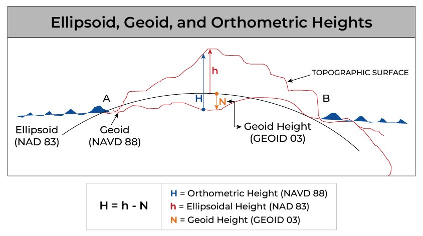
A challenge comes when transforming ellipsoidal vertical datums into orthometric vertical datums. This conversion requires using a geoid height model, a conglomeration of ellipsoidal heights between an ellipsoidal datum and a geoid. As a result, the geoid height models get directly tied to the geoid and ellipsoid that define them. As shown below, the orthometric height equals the difference between the ellipsoidal and geoid heights.
Projection Coordinate Frames and Systems
At this point, we have discussed what a geographic coordinate system is. It is a 3D coordinate system defined by a datum or a reference frame used to model the Earth’s shape. But what’s the difference between a geographic coordinate system (GCS) and a projected coordinate system (PCS)?
In summary:
- A GCS tells us where data is located on the earth’s surface (3D);
- A PCS tells the data how to draw the data on a flat surface, like a paper map or a computer screen.
Unlike some geographic coordinate systems (GCS), projection coordinate systems (PCS) are defined on a flat, two-dimensional surface. This means that values such as lengths, areas, and angles will remain constant across the plane.
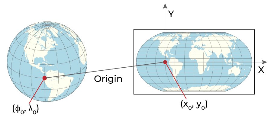
While on a flat surface, all projection coordinate systems are based on a sphere or spheroid coordinate system. As shown below, locations in a projected coordinate system give linear “x” and “y” values representing easting and northing coordinates on a consistent and evenly spaced grid.
The most common types of projections are conic, cylindrical, and planar. A forecast is made by creating points or lines of contact called points or lines of tangency. In the case of a planar projection, only one point of tangency is required. Tangential cones and cylinders contact the globe on a string. If the projection surface intersects through the world, the resulting projection is a secant instead of a tangent. Lines of contact are essential because they define locations that have no distortion. An example is the central meridian, along with standard parallels called the standard line. Distortion increases as you get further away from the line of contact.

An excellent example is the Universal Transverse Mercator (UTM) projection, used in Inertial Labs’ PCMasterGL software. UTM stands for the Universal Transverse Mercator, a type of map projection. This projection uses cylindrical coordinates and turns the Earth’s curved surface into a flat one. It allows us to measure distances accurately across large areas. The UTM projection of the transverse cylinder rotates in 6-degree longitude increments, which creates 60 strips called projection zones. Each of these 60 zones is projected onto a plane separately to minimize scale distortion in each zone. This central meridian runs north-south through the middle of each location, dividing it into two halves. It’s like a line that stretches up and down, helping you to navigate your way around.
Furthermore, these zones are divided into 8-degree latitude increments, resulting in 20 bands labeled with letters. So, with a few exemptions, the UTM zones are divided into “boxes” 6 degrees in longitude by 8 degrees in latitude. Each zone consists of a number followed by a letter to identify areas of the world corresponding to a site quickly. For example, Zone 32V covers the west coast of Norway.

The Next Step, Analysis
For many applications, classifying points is one of the first steps in post-processing any point cloud. Point classification is the process of identifying the type of object that the point is reflecting off. So, for instance, if a laser pulse gets reflected off a tree, the resultant point could be classified as vegetation. Point classification categories can be as broad as ground vs. non-ground or as specific as the type of structure/feature the laser pulse reflected.

Point classification algorithms group points together based on their spatial-based and echo-based features. A LiDAR point’s spatial features consider the point’s environment, height features, eigenvalue features, local plane features, plane slope, and more. Echo-based features, such as terrain-echo, vegetation-echo, and others, are determined using the return pulse from the surface. The return number (first, second, last, and others) also plays a role in determining a pulse’s echo-based features. One or both of these features are integral in the accurate automatic classification of vegetation, buildings, and ground surfaces.
Point classification provides the foundation for creating DTM, DEM, and DSM models. Point classification makes it easy to get only bare earth data for DEMs and DTMs while allowing DSMs to start by including points from manufactured and natural features.
DTM, DSM, and DEM
A DTM provides a digital description of a surface with heights set over two-dimensional points on a reference surface. This reference surface can be an ellipsoidal, geoidal, or mean sea level height or a geodetic datum. These unique heights are approximate values between these points and a reference surface. DTMs only represent the bare ground of the terrain and therefore do not measure vegetation sizes or manufactured features. DTMs are often mathematically represented as 2D raster or matrix grids, irregularly distributed 2D points, 1D profiles, contours/lines of constant elevation, and Fourier series. DTMs can calculate derived values such as volumes, slopes, contours, drainage, and gravitation attraction. Values like these are instrumental in planning roads, railways, drainage, inundations, and much more.
Like a DTM, a DSM is a collection of points with different height values. The main difference between a DSM and a DTM is that a DSM comprises more than bare Earth heights. Heights also come from natural and manufactured features, becoming especially useful in vegetation management applications as one can see where and to what extent vegetation encroaches on a structure like a utility line. It is also helpful in urban planning applications as DSMs can determine how proposed buildings would obstruct the view of city residents.
A Digital Elevation Model (DEM) is a raster grid of the bare earth referenced to a vertical datum. DEMs only contain ground points and exclude manufactured and natural structures. Formally derived from topographic maps, DEMs are increasingly becoming derived from high-resolution LiDAR. Since DEMs are a collection of ground points with varying height values, they are especially prevalent in hydrology in delineating watersheds and calculating flow direction and accumulation. DEMs are also helpful for analyzing terrain stability in high-slope areas and providing valuable information for users looking to enact structures like highways or buildings.

Contours
Since LiDAR data provides highly accurate height data for each of its points, users can create detailed contour maps. A contour map consists of multiple contour lines. Each line represents a line of equal elevation/height compared to a reference like mean sea level (MSL). As a result, a contour map allows us to see differences in elevation between successive contour lines. In turn, this allows the user to view the vertical profile of the mapped environment.
Tree and Forestry Analysis
With LiDAR’s ability to penetrate vegetation with multiple return pulses, LiDAR point clouds are instrumental in producing a 3D forest model from the canopy to the ground beneath it. This ability to visualize the forest canopy and the ground simultaneously is a massive advantage of LiDAR. In the past, land managers had to rely on topographic maps for ground classification and field surveys to obtain tree volumes and height information.
LiDAR Data and Post Processing of LiDAR Data allows users to obtain the following items:
- Digital Elevation Models (DEM)
- Tree heights and digital surface models
- Crown cover
- Forest structure
- Crown canopy cover
- Volume – Canopy geometric volume
- Biomass – Canopy cover
- Density – Height-scaled crown openness index and counts of delineated crowns
- Foliage projected cover – Crown dimensions
Using LiDAR data, forest inventories can be collected at the single tree level more precisely. LiDAR has typically been used in forestry to retrieve primary structural attributes, such as tree height, canopy cover, and vertical profiles. These statistics can be, in turn, used to compute basal area, timber volume, biomass for alternative energy, and carbon sequestration analysis.

The vegetation management software takes 3D point clouds and rapidly analyzes them to find locations and measurements of vegetation encroaching on powerline assets. This data can be communicated as a classified LAS point cloud, map icons, or SHP files.
How RESEPI Can Transform Your Business
Construction
Point clouds and subsequent models generated from RESEPI can aid construction projects by providing information and analysis, assisting in creating simulations when developing a project, and helping determine repair and maintenance requirements for every project. With LiDAR’s capability of producing multiple return data, RESEPI can penetrate vegetation and get ground points, even in covered areas. With this in mind, construction companies can plan by retrieving a terrain map of a construction site, even in dense environments.

Bare earth models, or DTMs, are instrumental in the planning stage of a construction project. Raw earth models derived from Lidar data allow construction planners to assess land stability by removing natural and manufactured aboveground structures. Users can consider the risk of landslides and flooding by analyzing slope gradients.

Utilities
As required by law, regular inspections significantly reduce the frequency of power outages and provide valuable data to prevent fires caused by faulty overhead utility lines. Traditionally, utility lines have been inspected using on-the-ground methods that often prove to be labor-intensive and require surveyors to be physically present along the length of the utility network. Drone-based LiDAR Point, Cloud Deliverable systems, can quickly map large utility networks and access difficult terrain areas. Point cloud post-processing provides meaningful geospatial data, like measuring the distance between the transmission line and vegetation, and a more accessible alternative to calculating distances with heavy measuring rods and theodolites.

Conclusion
In summation, data collected by LiDAR Point Cloud Deliverables can provide valuable metrics for various applications. From topographic mapping to asset inspection to site monitoring, the Inertial Labs RESEPI is a quick and efficient way to generate models of an environment. Beyond just making an excellent-looking 3D model, LiDAR can provide actionable data that offers immediate value to any inspection or mapping service. With the advances in modern LiDAR data, data can be displayed almost identically to how it appears in reality and provides comparable accuracy to field surveys. With the ability to perform customized analyses in line with the priorities and risks of an application, owners have the power to understand what needs to be done. With custom options and an outstanding price-performance ratio, Inertial Labs is working hard to provide high-quality solutions for various applications at an affordable price.
| RESEPI | |||
|---|---|---|---|
|
Weight |
0.37 kg (w/o LiDAR) |
||
|
Power Consumption |
0.5 cm (PPK) / 1cm + 1ppm (RTK) |
||
|
Position Accuracy |
<0.01º Pitch & Roll; <0.05º Heading |
||
|
Attitude Accuracy |
Velodyne VLP / QUANERGY / OUSTER / LIVOX |
||