White Papers

Abstract

Beginners using LiDAR for the first time often struggle to understand a point cloud and how to work with it. Therefore, this paper discusses a point cloud and how it is generated using LiDAR.

Here are the sections that will be covered: Introduction to Point Cloud, Step-by-step process for creating a Point Cloud, Additional data contained in the Point Cloud, Point Cloud data processing, Using Point Clouds. The conclusion will summarize the benefits of using Point Cloud.

Section 1. Introduction to Point Cloud

               A point cloud is a collection of vertices in a three-dimensional coordinate system. These vertices are typically defined by coordinates (X, Y, Z) and generally are intended to represent the exterior surface of an object [1]. Point clouds are created by 3D scanners, most often LiDAR or Time of Flight (ToF) cameras [2]. 3D scanners automatically measure many points on the surface of the scanned object and usually generate a point cloud as a digital data file. Thus, a point cloud is a set of points obtained from 3D scanning an object, Figure 1.

Figure 1. A teapot in the form of a point cloud.

Point clouds are used for many purposes, including creating three-dimensional models (meshes), monitoring power lines and forests, and surveying autonomous vehicles and robots [3]. Point clouds are one of the sources for creating a Digital Elevation Model or a Digital Terrain Model [4].

               Now, let’s look at how point cloud generation systems work. ToF laser cameras are part of a broader class of non-scanning lidars in which each laser pulse captures the entire scene [2]. The simplest version of a ToF camera uses light pulses or a single light pulse. The lighting is turned on for a very short time; the resulting light pulse illuminates the scene and is reflected by objects in the field of view. The camera lens collects the reflected light and displays it on the sensor.

               LiDAR works similarly. When a LiDAR laser beam hits an object, such as a tree or building, some of the light is reflected from the sensor [5]. By accurately timing the return of each laser pulse, the LiDAR system can determine the distance to each reflected point. These calculations are based on the time-of-flight (ToF) method, which assumes a constant speed of light.

LiDAR and TOF (Time-of-Flight) sensors are distinguished primarily by their accuracy and range. LiDAR provides centimeter-level accuracy and is excellent for long-range applications such as autonomous vehicles. TOF sensors are more compact, suitable for short- and medium-distance applications, and consume less power. In this article, we will consider the construction of a point cloud based on LiDAR scanners.

Section 2. Step-by-step process for creating a point cloud

Let’s look at the process of obtaining a point cloud using LiDAR. The general operating principle determines the range, measuring the time light travels from the emitter to the object and back to the receiver, as shown in Figure 2. Mathematically, this is expressed in a simple formula:

L = c * t / 2

where L is the distance from the lidar to the object, c is the speed of light, and t is the flight time.

Figure 2. The time of travel of the light pulse reflected from the target.

               After the pulse of light has returned to the receiver and the distance to the object has been determined, the point’s coordinates (X, Y, Z) are recorded in the file. This process is conventionally shown in Figure 3.

Figure 3. Determining the coordinates of the object.

In this case, the coordinates of the object can be determined using the following formulas:

Where r is the distance from the sensor to the object; α and β are the angles of the deflection system from the horizontal and vertical, respectively.

Then, these coordinates are converted into geographical coordinates. How this happens can be found in this paper [6]. Suppose the LiDAR system is used without satellites in the so-called offline mode. The data is collected in a local coordinate system, and navigation is carried out using SLAM algorithms [7].

It is important to note that there are single-beam and multi-beam lidars. Single-beam lights have a single light source directed by a deflection system, as shown in Fig. 3. Multibeams have many sources. Today, a trendy solution is to have multiple sources in a vertical channel that can rotate 360 degrees on the horizon, as shown in Fig. 4.

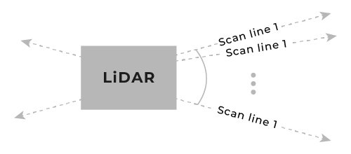Figure 4. Many modern lidars have several lasers in a vertical channel.

Thus, in one rotation in the horizontal plane, it is possible to collect many points, due to which objects are scanned with greater detail. The more vertical channels, the denser the cloud and the more detailed the objects will be, Figure 5 [8].

Figure 5. Dependence of detail on the number of vertical channels.

               Modern LiDAR systems have the architecture shown in Figure 6. A GPS-Aided INS comprises an inertial measurement unit (IMU) containing three-axis accelerometers, gyroscopes, and a GNSS receiver. After initial orientation and bias estimation, data from the IMU and GNSS receiver get fed through a robust Kalman filter algorithm, in which the unit will begin outputting correct and accurate orientation, position, velocity, and timing. In the scope of a LiDAR payload, the INS is essential for precise data georeferencing. Georeferencing applies a coordinate system to the point cloud to relate accurately to a geographic (or local) coordinate system. The GNSS receiver is responsible for obtaining a known global position of the rover to which the payload is mounted. The IMU is accountable for transferring that known position to the georeference of the acquired LiDAR data point. Add a data logger, and this system now logs point clouds consisting of issues that each have a location in space. The need for accurate georeferencing highlights the importance of a quality IMU, GNSS receiver, accurate boresighting (alignment of the LiDAR to the IMU), IMU-GNSS antenna offset calculation, and vehicle-payload rotation compensation [9]. These critical components and processes will result in an inaccurate point cloud if not carefully selected, calculated, and compensated for.

Figure 6. RESEPI payload architecture from Inertial Labs.

The part highlighted by red box 1 is the payload. It collects raw data during a flight or trip, which must then be processed to produce a point cloud. Blue Box 2 is the software installed on the user’s computer. Inertial Labs has developed a special software, PCMasterPRO, for data processing aimed at post-processing to increase accuracy [10]. However, there is also support for RTK correction using a particular modem. In addition, the system supports SLAM operation, so data collection does not require satellites.

Next, let’s look at the other data in the point cloud and how it can be helpful.

Section 3. Additional data contained in the Point Cloud

In addition to coordinates, LiDAR data contains information about the intensity of each point. In other words, it is information about how much light energy is returned to the receiver after the light pulse is reflected from the object. It depends on the material’s properties from which the object is composed. As you know, black objects, such as asphalt, rubber, and black paint, absorb infrared radiation better, so the intensity parameter for such points will be minimal. This value is often from 0 to 255, but it can vary for different lidars. This parameter helps you distinguish between materials or surface textures.

               Also, each point can contain additional information. Let’s consider the most useful for the user:

• Return number. When LiDAR emits a light pulse, it can be reflected multiple times, which the receiver will detect. This happens when the pulse is partially reflected from the object back to the receiver, but part of the laser pulse continues to hit another object or surface. Some lidars can register multiple returns (2 or more). Most often, numerous returns are characteristic of vegetation, Figure 7.

Figure 7. Multiple returns from the tree.

• This is the timestamp for each point when it was acquired. Most often, the timestamp is tied to the GPS time. The GPS receiver records the time value when the next point is received. According to the GPS time countdown, it is recorded as a reference to the beginning of the GPS week or the GPS epoch (midnight on January 6, 1980), Figure 8.

Figure 8. Point cloud colored according to GPS time.

• Points can be classified according to the surface from which the reflection occurred (e.g., ground, buildings, vegetation). The classification of point cloud data formats is determined by the corresponding fields or bits, as in Figure 9 [11]. The value for this attribute is not collected during data collection. The classification value parameter will be 0, corresponding to “Created, never classified.”

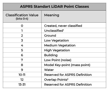Figure 9. Table of values and corresponding classes, according to the LAS 1.2 specification.

• RGB color. If a LiDAR system uses a camera to color a point cloud, the dot color value is set to the pixel’s RGB (red, green, blue) color. Cloud colorization occurs after data collection at the post-processing stage, Figure 10.

Figure 10. An example of a painted and unpainted point cloud.

The return number, timestamp, and classification data are handy for filtering clouds. Changing the GPS time values makes it easy to remove the noise accumulated while the LiDAR was stationary, Figure 8. After filtering, the cloud will take the form shown in Figure 11.

Figure 11. Filtered noise by timestamp.

In the same way, you can filter or highlight areas of interest for other parameters; for example, vegetation can be easily identified by the return number. However, we will not dwell on this in detail and will move on to consider the file formats of point clouds.

Point cloud formats

Today, there are many point cloud file formats; let’s consider the most popular ones:

• E57: A file with the .e57 extension is a compact, vendor-independent format used to store and share data for three-dimensional (3D) images, such as point clouds, photos, and metadata. Such data is often created using systems such as laser scanners. It was developed by the Data Interoperability Subcommittee of the ATSM E57 Committee on Three-Dimensional Imaging Systems. E57 is open source and stores 3D point data, their attributes (such as color and intensity), and 2D images obtained by the 3D imaging system [12].
• LAS: This binary file format is specifically designed to store lidar point cloud data. It was developed and maintained by the American Society for Photogrammetry and Remote Sensing (ASPRS) as a standardized format for lidar data exchange and interoperability. LAS files store detailed information about individual lidar points, including their three-dimensional coordinates (X, Y, and Z), intensity values, classification codes, and additional attributes that support both discrete and complete lidar data, allowing multiple return signals to be stored on a single laser pulse [11].
• LAZ: A highly compressed LAS file.
• PLY: A format for 3D polygons or meshes, vendor-neutral in design [13].
• PCD: This is a file format for storing 3D point cloud data. A format supported by the open-source Point Cloud Library [14].

In addition to the above, some lidar manufacturers have developed their proprietary file formats. The RESEPI software generates a cloud in the LAS format, so the user can use any point cloud software that supports this format. More on this below.

Section 4. Point cloud data processing

               Before using point clouds, let’s look at how data is preprocessed. After generating a point cloud, it contains, in addition to valuable and necessary information, noise.

For some tasks, it is valid and sometimes necessary to classify points to, for example, separate vegetation from buildings or road surfaces. 

               Third-party software is used for data processing: LiDAR360, TerraScan, CloudCompare, Global Mapper, etc. [15 – 18]. This software has many features for classification, filtering, and generation of digital maps, among many other tools. All of the examples below will be done using LiDAR360.

Cloud filtering is a straightforward, essential operation for removing noise. Before filtering, you can thin the cloud to reduce the number of points. You don’t need a cloud that is too dense to determine the shape, and the processing time for thinned data is significantly reduced. Figure 12 shows a cross-section of a point cloud in its original raw form. It shows a cross-section of a fence and a road. As you can see, there is noise in the form of individual points.  as shown in Figure 12 b. Less noise and a lower density of points can be observed here. Finally, the filtered cloud after thinning the data is shown in Figure 12 c.

a	b	c

Figure 12. Examples of point cloud filtering are a source cloud, b thinned cloud, and a thinned and filtered cloud.

               After thinning and filtering, the noise was removed entirely, the cloud became less dense, and there were enough points to convey the shape of objects and the relief of the road surface. Processing parameters are deliberately not given here since they are selected based on the data requirements.

               The following necessary procedure is the Classification of objects. It is necessary to separate groups of points from each other quickly. For example, vegetation or buildings from the road surface. This is a crucial task because, in many respects, the construction of digital maps of relief or surface depends on the preliminary classification of objects.

               For example, let’s take a simple cloud and separate from it the points that form the road surface, Figure 13.

Figure 13. A cloud of dots with coloring by height.

After thinning and filtering the noise, we get the result shown in Figure 14.

Figure 14. Point cloud after classification.

The program classified the points, separating those that form the road from the rest. Buildings, vegetation, etc., are classified in the same way.

Now that we’ve looked at the basic operations with point clouds let’s look at how they can be used to solve real-world problems.

Section 5. Using point clouds

Obtaining a Digital Terrain Model from a point cloud is also easy. Let’s show this using the example of an estuary scanning project [19]. The result is shown in Figure 15 (right). To do this, you must classify the points and select the settings. The less spacing, the more detailed the map will be. It is worth noting that this article deliberately does not provide numerical values of processing parameters because they will vary from cloud to cloud. Programs can select the parameters automatically, which is enough for most tasks, but sometimes, it takes several iterations to choose the parameters to achieve a good result. In this case, the default parameters were used for demonstration purposes only; more details about the parameters can be found in the datasheet.

Classified cloud visualized by height	The TIN surface created from a DTM mesh with 0.3 m spacing

Figure 15. Digital Terrain Model.

Generating a 3D model is just as simple. Let’s demonstrate using the example of Hanbit Tower. «Hanbit Tower, standing tall at 93 meters, is a symbolic sculpture commemorating the 1993 World Expo, a landmark event in the history of the Republic of Korea. Its design embodies light, science, and space, representing a beacon of hope that bridges the past, present, and future. The name “Hanbit,” meaning “a ray of light,” encapsulates the wisdom of yesteryears, connecting it with the infinite possibilities of the future» [20]. Hanbit Tower is shown in Figure 16.

Figure 16. Hanbit Tower.

After collecting the data, the cloud was processed to obtain a 3D model, Figure 17.

Figure 17. Point cloud (left) and 3D model (right).

For the second example, the building of the Kyiv Polytechnic Institute was used – an institution of higher education of engineering profile, founded in Kyiv in 1898; today, it is one of the largest universities in Ukraine in terms of the number of students with a wide range of specialties and educational programs for training specialists in technical and humanitarian sciences, Figure 18. In this case, the corridor of the old building with the architectural characteristic of that time was scanned, and the scanning was carried out in SLAM mode. The result was a point cloud, Figure 19, which was also converted into a 3D model, Figure 20.

Figure 18. Corridor.	Figure 19. Point cloud.

Figure 20. 3D model of the corridor of the old building.

Thus, using lidar, it is easy and quick to collect the necessary data and convert it into a 3D model, which can then be used for various purposes, for example, blanks for new design solutions.

               After we have answered the question “how to create a point cloud” and considered simple operations with it, let’s get acquainted with the possibilities that RESEPI can provide to the user.

Section 6. RESEPI

               RESEPI™ (Remote Sensing Payload Instrument) is a sensor-fusion platform for accuracy-focused remote sensing applications [21]. RESEPI utilizes a high-performance Inertial Labs INS (GPS-Aided Inertial Navigation System) with a tactical-grade IMU and a high-accuracy single or dual-antenna GNSS receiver, integrated with a Linux-based processing core and data-logging software. The platform also provides a WiFi interface, optional imaging module, and external cellular modem for RTCM corrections. RESEPI can be operated by a single hardware button or from a wirelessly connected device via a simple web interface. Figure 21 shows the RESEPI range with different lidars to cover a wide range of user needs.

Figure 21. Comparison of RESEPI models.

               Thanks to a wide range of different lidars, the user will not overpay if the accuracy is enough, for example, 4-5 cm.

In the remote sensing industry, many different terms get thrown around about accuracy. In general, any accuracy specification can fall under either relative accuracy or absolute accuracy. In the context of a complete LiDAR payload, relative accuracy measures the accuracy between points relative to each other within a single project. Absolute accuracy measures how close a measured value is to a known, surveyed location (actual value) in a geographic coordinate system. An example of how relative accuracy and absolute accuracy are calculated is shown in the figure below. This is an important distinction when analyzing the quality of LiDAR remote sensing solutions, as these values speak to the quality of different components of the remote sensing payload. Relative accuracy is more dependent on the LiDAR scanner, while absolute accuracy is more dependent on the quality of the inertial navigation systems (INS) on board. Both parameters are essential for surveying applications to get the job done correctly, as shown in Figure 22.

 Figure 22. Relative vs Absolute Accuracy.

To improve data quality, PCMasterPro implements a PPK post-processing solution that automatically reduces errors associated with GPS and INS, allowing for position accuracy of about 0.5 cm, Heading accuracy of 0.03 ^o, and Pitch/Roll accuracy of 0.006 ^o, Figure 23.

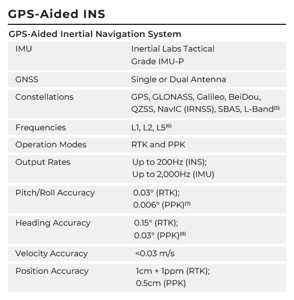Figure 23. Accuracy of orientation and position angles.

Let’s look at the example of RESEPI M2X to see what accuracy the user gets at different altitudes relative to ground level [22]. For this purpose, three flights were made at various altitudes, the results of which are shown in Figure 24 and Table 1.

	50m AGL
	100 m AGL
	150 m AGL
Figure 24. RESEPI M2X Relative Accuracy.

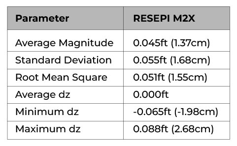Table 1. RESEPI M2X Absolute Accuracy.

LiDAR is a powerful technology that allows users to capture an environment in detail and with high accuracy while saving man-hours and reducing the safety risk of the survey team. LiDAR payloads can produce insightful deliverables such as DEMs, DSMs, and hillshade models that give the end user actionable results.

Conclusion

               A point cloud is a convenient and practical way to represent the environment in three dimensions. This paper considers a point cloud and how it is formed. LiDAR measures the distance to objects in the form of a set of points and assigns each point a corresponding coordinate. Thanks to INS integration, the coordinates are georeferenced.

The raw LiDAR data is post-processed using special software to form a point cloud, which a camera can also color. Then, using third-party software to work with point clouds, the user can easily and quickly get digital maps or 3D models from them, as demonstrated in the examples. The procedure of point cloud preparation – data filtering and subsampling, as well as what file formats are available – is considered. The advantages of using RESEPI for the user are highlighted.

Inertial Labs is committed to providing high-quality solutions with customization and excellent value for money at an affordable price.

References

[1] Wikipedia Contributors. “Point Cloud.” Wikipedia, Wikimedia Foundation, 8 Dec. 2019, en.wikipedia.org/wiki/Point_cloud.

[2] “Time-of-Flight Camera.” Wikipedia, 25 June 2020, en.wikipedia.org/wiki/Time-of-flight_camera.

[3] “7 Real-World Applications of LiDAR Technology – DFRobot.” Www.dfrobot.com, www.dfrobot.com/blog-1644.html.

[4] Team, LuxCarta. “Understanding DEM vs DTM vs DSM: Which Mapping Model Is Right for You?” Luxcarta.com, LuxCarta SARL, 22 Feb. 2024, www.luxcarta.com/blog/dem-dtm-dsm. Accessed 3 Sept. 2024.

[5] Wikipedia Contributors. “Lidar.” Wikipedia, Wikimedia Foundation, 13 Oct. 2019, en.wikipedia.org/wiki/Lidar.

[6] INS + LIDAR

[7] Wikipedia Contributors. “Simultaneous Localization and Mapping.” Wikipedia, Wikimedia Foundation, 8 July 2019, en.wikipedia.org/wiki/Simultaneous_localization_and_mapping.

[8] Hesai Webmaster. “Things You Need to Know about LiDAR: The More Lasers, the Better? | HESAI.” HESAI, 20 Mar. 2023, www.hesaitech.com/things-you-need-to-know-about-lidar-the-more-lasers-the-better/. Accessed 3 Sept. 2024.

[9] Mendez, Maria. “A Comprehensive Guide to Boresight and Strip Alignment for LiDAR Data Accuracy.” Inertial Labs, 16 Aug. 2024, inertiallabs.com/a-comprehensive-guide-to-boresight-and-strip-alignment-for-lidar-data-accuracy/. Accessed 3 Sept. 2024.

[10] Inertial Labs. “RESEPI Quick-Start Guide – Setting up Your LiDAR Survey System and PCMaster – Inertial Labs.” YouTube, 4 Aug. 2022, youtu.be/AygQTBVNrKw. Accessed 3 June 2024.

[11] LAS Specification. https://www.asprs.org/a/society/committees/standards/asprs_las_format_v12.pdf

[12] SIMON, Vincent. “E57: Exploring the Cloud of Points Format – Benefits and Extensibility.” Cadinterop.com, 2024, www.cadinterop.com/en/formats/cloud-point/e57.html#:~:text=The%20E57%20file%20format%20is. Accessed 3 Sept. 2024.

[13] “PLY (File Format).” Wikipedia, 22 June 2023, en.wikipedia.org/wiki/PLY_(file_format).

[14] “The PCD (Point Cloud Data) File Format — Point Cloud Library 1.14.1-Dev Documentation.” Pointclouds.org, 2024, pointclouds.org/documentation/tutorials/pcd_file_format.html. Accessed 3 Sept. 2024.

[15] “LiDAR360 Software and Real-Time Point Cloud Display.” Www.greenvalleyintl.com, www.greenvalleyintl.com/LiDAR360/.

[16] “Terrasolid – Software for Point Cloud and Image Processing.” Terrasolid, 21 Sept. 2023, terrasolid.com/.

[17] “CloudCompare – Open Source Project.” Www.danielgm.net, www.danielgm.net/cc/.

[18] “Global Mapper.” Blue Marble Geographics, www.bluemarblegeo.com/global-mapper/.

[19] Mendez, Maria. “Integrating RESEPI Technology for Advanced Estuary Mapping.” Inertial Labs, Aug. 2024, inertiallabs.com/integrating-resepi-technology-for-advanced-estuary-mapping/. Accessed 3 Sept. 2024.

[20] “Illuminating Hope: The Hanbit Tower Christmas Project of (Korea, 2020).” MatrixWorks Europe, 26 Mar. 2024, matrix-works.eu/knowledge-base/illuminating-hope-the-hanbit-tower-projection-mapping-in-korea/. Accessed 7 Aug. 2024.

[21] “RESEPI – LiDAR Payload & SLAM Solutions.” RESEPI, 12 July 2024, lidarpayload.com/.

[22] Mendez, Maria. “WISPR Accuracy Study – RESEPI M2X vs. XT-32.” Inertial Labs, 15 Dec. 2023, inertiallabs.com/wispr-accuracy-study-resepi-m2x-vs-xt-32/.