Overview
The article reveals the key differences between map projections and coordinate systems, two fundamental concepts of geodesy and cartography. The reader will learn the main differences between the projections and their applications. Many illustrations are provided for better understanding.
Special attention is given to the transformations between different coordinate systems, their impact on accuracy and data compatibility, and the importance of choosing the correct projections and coordinate systems for various tasks. Attention is paid to modern software solutions that simplify work with projections and coordinates, helping professionals solve complex problems efficiently. An example of using modern PCMaster Pro software for point cloud reprojection is given.
Here are the sections that will be covered: “Introduction to Map Projections and Coordinate Systems”, “Transformation between datums. Why is it necessary?”, and “PCMaster Pro from Inertial Labs“. The conclusion will summarize the benefits of using different projections and modern software solutions for transformations.
Section 1. Introduction to Map Projections and Coordinate Systems
What is a coordinate system?
In geodesy, a coordinate system describes the position of points on or near the Earth. The choice of a coordinate system depends on the tasks, such as mapping, engineering, navigation, or astronomical observations.
There are the following types of geodetic coordinate systems:
- Geocentric coordinate system: A three-dimensional system originating at the Earth’s center of mass. Applications: Global navigation (GNSS), satellite geodesy [1].
- Geographic coordinate system: A system in which the position of a point is determined by latitude, longitude, and elevation. Applications: Cartography, navigation [2].
- A flat rectangular coordinate system (projected) displays coordinates on a flat surface. It uses map projection to convert from a spherical surface of the Earth to a plane. Its applications include engineering, construction, and cadastre [3].
- Local coordinate system: A system with a coordinate origin at a specific point on the ground—application: Construction, mining, and local engineering tasks [4].
There are also altitude coordinate systems:
- Ellipsoidal height. This is the height relative to the mathematical ellipsoid used in the datum. It is used in satellite navigation systems (GPS).
- Geoidal altitude. This is the height relative to the geoid (mean sea level). It is used in surveying and construction.
- Orthometric Height (H). It is the difference between the vertical distance from a location on the Earth’s Surface and the geoid.
The difference between heights is shown in Figure 1.

Figure 1. Height differences.
Cartographic projections: what it is and why they are needed.
Cartographic projections are mathematical ways of displaying the surface of the Earth (or other celestial bodies) on a plane [5]. The Earth has a shape close to an ellipsoid, and converting its surface into a flat image inevitably introduces distortions. Projections are created to minimize these distortions, depending on the map’s purpose [6].
Projections can distort:
- Shape (angles between lines, such as the shape of continents).
- Area (e.g., the ratio of sizes of different pieces of land).
- Distances (the length of lines between points).
- Directions (azimuths, angles between directions).
Thus, projections are also divided according to the method of distortion:
- Equal area: preserves areas but distorts shapes. They are used for thematic maps where the relative sizes of regions are essential. An example of such a projection is the Mollweide projection, as shown in Figure 2 [6].

Figure 2. World map in the Mollweide projection.
- Equirectangular: preserves shapes and angles in small areas but distorts areas. They are used for maritime navigation. For example, the well-known Mercator projection is shown in Figure 3 [6].

Figure 3. Mercator projection map of the world.
- Equidistant: partially preserves distances—for example, the Eckert projection, as shown in Figure 4 [6].

Figure 4. Map of the world in the Eckert projection.
- Azimuthal: they preserve the accurate directions (azimuths) from the center point of the projection to any other point on the map (e.g., used for navigation), as shown in Figure 5 [6].

Figure 5. World map in Azimuthal Equidistant Map Projection.
Projections are categorized by their geometric basis as follows:
- Cylindrical: created by projecting the Earth’s surface onto a cylinder. Suitable for displaying the entire Earth, as shown in Figure 6.
- Conical: uses a cone. Suitable for mid-latitude maps, as shown in Figure 6.
- Azimuthal (flat): based on projecting a surface onto a plane. Suitable for maps of polar regions or small areas, as shown in Figure 6.

Figure 6. The Cylindrical, The Conical, and The Azimuthal Projections.
- Pseudoconical: the parallels are represented by arcs of concentric circles, one of the meridians, named the mean, is a straight line, and the others are curves symmetrical about the mean. An example of a pseudoconical projection is the equal-sized Bonnet pseudoconical projection, as shown in Figure 7 [6].

Figure 7. World map in Bonnet projection.
- Pseudocylindrical: In pseudocylindrical projections, all parallels are represented by parallel lines, the middle meridian by a straight line perpendicular to the parallels, and the other meridians by curves. The middle meridian is the axis of the projection’s symmetry. One famous example of a pseudocylindrical projection is the Mollweide projection.
- Polyconic: In polyconic projections, the equator is represented by a straight line, and arcs of eccentric circles represent other parallels. Meridians are depicted by curves symmetrical about a central straight meridian perpendicular to the equator. One of the best-known examples is the American Polyconic Projection, as shown in Figure 8 [6].

Figure 8. American Polyconic Projection.
Besides those mentioned above, other projections do not belong to the types discussed above. However, we will not dwell on them in detail but move on to the examples.
Examples of popular projections:
- Mercator projection: popular for navigation because it preserves angles. But it distorts dimensions. Greenland appears much larger than it is [7].
- Robinson projection: balances distortions, often used to display the entire Earth [8].
- Lambert projection (conic conformal): widely used for aviation and regional maps [9].
- Gauss-Kruger projection: used in geodesy and for topographic maps [10].
- UTM: Unlike the Gauss-Kruger projection, UTM uses a scale factor of 0.9996. As a result, in this projection, the scale factor of one is not located on the central meridian line, but at some distance (about 180 km) on either side of it. Due to this, the maximum distortion within a six-degree zone does not exceed 0.1% [11].
The choice of a particular projection depends on the purpose of the map, for example:
- Geographic maps of the world: compromise projections (Robinson, Winkel-Tripel).
- Thematic maps: equal-area projections.
- Marine and aviation maps: conformal projections.
- Maps of small areas: minimal distortions (for example, local azimuthal projections).
It should be noted that it is impossible to eliminate distortions, so there is no “perfect” projection. Cartographers choose a projection that minimizes a particular type of distortion depending on the tasks. With the development of technology, specialized software allows you to select and configure projections for specific tasks automatically.
Now we will move on to a fundamental concept of “Datum”. Datums consider local features of the Earth, such as surface irregularities, due to which coordinates become more accurate [12].
A datum (or geodetic reference system) is a system that determines the position of objects on Earth. It links a mathematical model of the Earth (an ellipsoid) to the real surface so that the coordinates of points on a map can be uniquely determined.
The main elements of a datum are:
- Ellipsoid: A mathematical model of the shape of the Earth used for calculations (e.g., WGS84, GRS80, Clarke 1866). Ellipsoids vary in size and degree of flattening to better match the shape of the Earth in different regions.
- Datum: Each datum defines a specific point on the Earth that serves as the basis for all calculations. For example, the NAD27 datum is based on a fixed point in Kansas, USA.
Datums can be global or local. Global ones describe the entire Earth (e.g., WGS84), while local ones are used for specific regions where they provide the greatest accuracy (e.g., NAD27).
Thus, the coordinates (latitude, longitude, and altitude) depend on the selected datum. Different datums can give different values for the same physical point on Earth. For example, a point located in a specific place can have different coordinates in the WGS84 and NAD27 systems, since the ellipsoids and reference points differ.
The choice of datum depends on the tasks being solved; for example, WGS84 is used for navigation using GPS, and in geodesy, local datums (such as NAD83) are used for detailed measurements.
Section 2. Transformation between datums. Why is it necessary?
Coordinate transformation converts coordinate information from one reference system (datum) to another. For example, LiDAR Payloads, such as RESEPI [13], are widely used today for mapping and monitoring purposes. Navigation systems for such payloads mainly use WGS84, followed by a point cloud projection in UTM (although this is not an axiom).
Since accuracy is critical for mapping, geodesy, and cadastral purposes, it is necessary to convert coordinates between different datums. This uses various methods, such as the Helmert or Molodensky transformation [14].
Basic transformation methods
1) Translation
This is the simplest method using three shifts ![]() .
.

It is used for simple transformations when the difference between datums is minimal. For example, when switching between local datums that use similar ellipsoids.
2) Helmert transformation
A more complex method that includes translation, rotation, and scaling. It considers the change in the position and orientation of the ellipsoid.
This transformation requires three simple steps:
- For datum A, it is necessary to convert geodetic coordinates (Latitude, Longitude, Height) into ECEF coordinates (X, Y, Z)
- Using parameters, convert the ECEF coordinates of datum A to the datum B coordinates
- Convert ECEF coordinates of datum B into geodetic coordinates

![]() the three translations;
the three translations; ![]() minimal rotation angles;
minimal rotation angles; ![]() the scale factor.
the scale factor.
It is used in complex transformations between different datums, such as NAD27 to NAD83 or Pulkovo 1942 to WGS84.
There is also an extended version of the Helmert transformation with fourteen parameters, with a linear time dependence for each parameter, which can be used to observe the time change of geographic coordinates due to geomorphic processes such as continental drift and earthquakes. It has been translated into software such as the Horizontal Time Dependent Positioning (HTDP) tool in the U.S. NGS software [15].
3) Molodensky-Badekas transformation
Three additional parameters can be used to get the new XYZ center of the reversal closer to the transformed coordinates to eliminate the relationship between offsets and reversals of the Helmert transformation. This transformation with ten parameters is called the Molodensky-Badekas transformation and should not be confused with the simpler Molodensky transformation.

![]() shift in X, Y, Z axes;
shift in X, Y, Z axes; ![]() rotation origin.
rotation origin.
The Molodensky-Badekas transformation is used to convert local geodetic datums to global datums such as WGS 84. Unlike the Helmert transformation, the Molodensky-Badekas transformation is irreversible because the origin of the reversal is referenced to the original datum.
4) Grid-based Transformations
A modern approach that considers small-scale changes in coordinates. Correction grids describe the difference between datums at each point in the region, for example, NADCON (North America) [16].
A simple shift is suitable for tasks where high accuracy is not critical. Helmert or Molodensky-Badekas transformations are used for more accurate transformations. Grid transformations give the highest accuracy when working in local coordinate systems.
Thanks to the development of technology, today, there is no need to know about such formulas and other mathematical studies. Software products such as PCMaster Pro enable coordinate transformations from one coordinate system to another in a few clicks. To better appreciate the simplicity of working with the software, you can watch a short video at this link [17].
In the next section, we will look at how to convert coordinates easily using PCMaster Pro.
Section 3. PCMaster Pro from Inertial Labs
Correct coordinate conversion is crucial for LiDAR data, especially from payloads. Such systems typically produce data in the WGS84 UTM coordinate system (the default for RESEPI data processing), which is ideal for global use. Although the WGS84 UTM system is widely used for obtaining LiDAR point clouds, it may be necessary to convert to local coordinate systems for further work (for example, in cadastral or cartographic tasks).
For this purpose, special software for RESEPI data processing (PCMaster Pro) was added to easily and quickly convert point clouds from WGS84 UTM to any other coordinate system and choose a suitable geoid for a particular region. The program automatically determines the list of datums available for a given area. This means that if the data was recorded in the USA, the user cannot select a local datum that is used, for example, in Italy (because it makes no sense).
Let’s consider an example of how to convert coordinates from WGS84 UTM to NAD83(HARN). Figure 9 shows the project after processing, as shown in the “Status” field, which shows UTM coordinates: E = 273650.647, N = 4336538.134, U = 159.756. To convert, click on “Settings” -> “Coordinates” menu, Figure 10, and in the opened window select from the list of horizontal and vertical models, Figure 11. After transformation, our point cloud has a new georeferencing and is ready for export and further processing (Figure 12).

Figure 9. Project after processing.

Figure 10. Utility for coordinate transformation.

Figure 11. Selecting a new coordinate system.

Figure 12. Reprojected point cloud.
Investing in quality data processing software will not only improve the accuracy of your results but will also make it easier to integrate LiDAR point clouds into your projects!
Conclusion
Understanding the differences between map projections and coordinate systems is key to successfully working with geospatial data. Cartographic predictions allow you to transform the Earth’s surface into a usable flat map, although this inevitably involves distortion. Coordinate systems, in turn, provide a uniform way of accurately locating objects in space.
To work effectively with geodata, it is vital to choose the correct projections and coordinate systems depending on the goals of the project and the region. Using modern tools and technologies that combine automation of transformations and work with projections allows us to minimize errors, save time, and achieve high accuracy. As we have shown with an illustrative example, it is fast and straightforward. Ultimately, a conscious approach to these aspects is essential for quality performance in geodesy, cartography, and related fields.
If you are involved in cadastral surveying, cartography, or on projects that require point cloud processing, using advanced coordinate transformation software will make your work easier and the results more accurate and of higher quality. Choosing the right technology is the key to a successful project.
References
[1] “Earth-Centered, Earth-Fixed Reference Frame.” W.wiki, Wikimedia Foundation, Inc., 20 June 2006, w.wiki/93uc. Accessed 8 Jan. 2025.
[2] “Geographic Coordinate System.” Wikipedia, 12 May 2020, en.wikipedia.org/wiki/Geographic_coordinate_system.
[3] Wikipedia Contributors. “Map Projection.” Wikipedia, Wikimedia Foundation, 9 Sept. 2019, en.wikipedia.org/wiki/Map_projection.
[4] “Local Coordinates.” Wikipedia, 5 Nov. 2021, en.wikipedia.org/wiki/Local_coordinates.
[5] Snyder, John P. “Map Projections: A Working Manual.” Pubs.usgs.gov, 1987, pubs.usgs.gov/publication/pp1395.
[6] “List of Map Projections.” Wikipedia, 11 Aug. 2020, en.wikipedia.org/wiki/List_of_map_projections.
[7] Wikipedia Contributors. “Mercator Projection.” Wikipedia, Wikimedia Foundation, 19 Dec. 2019, en.wikipedia.org/wiki/Mercator_projection.
[8] “Robinson Projection.” Wikipedia, 23 Aug. 2020, en.wikipedia.org/wiki/Robinson_projection.
[9] Wikipedia Contributors. “Lambert Conformal Conic Projection.” Wikipedia, Wikimedia Foundation, 22 Sept. 2019, en.wikipedia.org/wiki/Lambert_conformal_conic_projection.
[10] Wikipedia Contributors. “Transverse Mercator Projection.” Wikipedia, Wikimedia Foundation, 5 Aug. 2024, en.wikipedia.org/wiki/Transverse_Mercator_projection#Ellipsoidal_transverse_Mercator.
[11] “Universal Transverse Mercator Coordinate System.” Wikipedia, 10 May 2021, en.wikipedia.org/wiki/Universal_Transverse_Mercator_coordinate_system.
[12] Wikipedia Contributors. “Geodetic Datum.” Wikipedia, Wikimedia Foundation, 30 Dec. 2019, en.wikipedia.org/wiki/Geodetic_datum.
[13] “RESEPI – LiDAR Payload & SLAM Solutions.” RESEPI, 12 July 2024, lidarpayload.com/.
[14] “Geographic Coordinate Conversion.” Wikipedia, 24 Oct. 2021, en.wikipedia.org/wiki/Geographic_coordinate_conversion.
[15] US. “HTDP – Horizontal Time-Dependent Positioning.” Noaa.gov, 2025, www.ngs.noaa.gov/TOOLS/Htdp/Htdp.shtml. Accessed 8 Jan. 2025.
[16] US Department of Commerce, National Oceanic and Atmospheric Administration. “NADCON – North American Datum Conversion Utility – Tools – National Geodetic Survey.” Www.ngs.noaa.gov, www.ngs.noaa.gov/TOOLS/Nadcon/Nadcon.shtml.
[17] Garrison Wilson. “RESEPI LiDAR: How to Process in PCMasterPro.” YouTube, 18 Dec. 2024, www.youtube.com/watch?v=NDiecsMRAd0. Accessed 8 Jan. 2025.