1. Introduction and System Overview
Accurate positioning and orientation are fundamental to producing high-quality LiDAR point clouds and their deliverables in mobile and aerial mapping. Traditional single-antenna GNSS/INS configurations often struggle in environments with limited satellite visibility, resulting in degraded heading accuracy and positional drift. The use of a dual-antenna GNSS system directly addresses these challenges by providing stable, motion-independent heading and faster recovery from GNSS interruptions. This configuration ensures consistent data quality and reliability, even in dense or obstructed mapping environments.
This case study evaluates the performance of the Inertial Labs RESEPI GEN-II – a next-generation mobile mapping platform integrating a Dual Antenna INS-D and XT-32M2X LiDAR – to demonstrate its capability in achieving high-precision results under challenging GNSS conditions. Conducted in Paeonian Springs, Virginia, the study highlights how the dual-antenna configuration enhances trajectory accuracy, improves LiDAR point cloud consistency, and minimizes drift when compared to single-antenna setups. The results confirm that RESEPI GEN-II provides robust and repeatable performance for professional mobile mapping applications where reliability and precision are critical.
Dual Antenna GNSS in RESEPI
In our last paper, we have discussed the impact of the IMU as part of the system and its effect on the accuracy of point clouds [1] and their deliverables. Let’s take a look at Figure 1, which shows just some of the factors that affect the accuracy of the acquired data. As you can see, there are many, and it is not only the accuracy of the IMU that affects the point clouds.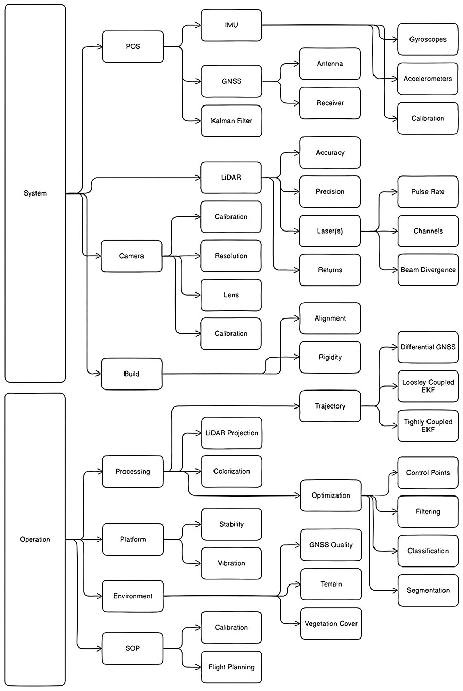
In this context, the choice between single or dual GNSS antennas becomes an important decision. The question may immediately arise: why pay more for a dual antenna system – doesn’t single antenna work just as well? Let’s consider the facts:
- A single GNSS-antenna cannot independently determine the heading of an object at rest – it requires motion and data from an inertial navigation system (INS). A dual-antenna system allows you to calculate heading directly, regardless of speed, by measuring the phase of the signal between the two antennas. This is especially important for precise orientation of the LiDAR scanner when starting, maneuvering or stopping.
- Dual GNSS in conjunction with the INS provides a more stable and accurate platform orientation measurement (pitch, roll, heading). This reduces the dependence on inertial measurement errors and reduces drift accumulation in the INS, especially in conditions with variable driving dynamics.
- In difficult conditions – near buildings, trees or other obstacles – the presence of two antennas helps to recover heading and orientation faster after GNSS signal loss, which is especially important for MMS (mobile mapping systems). Even in short-term shadows, the system can continue to correctly determine the platform’s orientation.
- With two GNSS antennas, it is easier and often times more accurate to calibrate offsets between GNSS, INS and LiDAR. This reduces point cloud alignment errors, reduces artifacts, and makes the point cloud more geometrically accurate.
Although a single GNSS antenna system may be cheaper, dual GNSS provides significantly higher orientation accuracy, which is critical for mobile LiDAR mapping. This is especially true for tasks that require centimeter accuracy and consistent data quality, such as engineering surveys, cadastral surveying, and high-precision mapping in complex urban environments.
Just for such tasks, Inertial Labs engineers have developed a dual-antenna system for MMS data acquisition as well as aerial mapping.
RESEPI GEN-II with XT-32M2X LiDAR
Experience superior aerial and mobile mapping with the RESEPI GEN-II, featuring the advanced XT-32M2X LiDAR (Figure 2). This system incorporates a lighter and longer-range version of the XT-32 scanner, enabling longer flights and higher operating altitudes (AGL) [2]. With an expanded vertical field of view (FOV), it’s ideal for efficiently surveying extensive regions, even those with dense vegetation. The RESEPI GEN-II stands out for its best-in-class data accuracy, extended detection capabilities, high point density, and overall adaptability.
The RESEPI GEN-II is an advanced, next-gen sensor-fusion platform built for high-accuracy remote sensing in aerial, mobile, and pedestrian (indoor, SLAM) applications. It leverages Inertial Labs’ Dual Antenna INS-D, featuring a Tactical Grade Kernel-210 IMU and an Extended Kalman Filter (EKF) for robust navigation both in real time and post-processed applications.
This system offers enhanced expandability, with capability for built-in software integrations via MAVLink and DJI’s Payload SDK (PSDK). Users benefit from new camera options with a wider FOV, faster shutter speeds, and higher resolution. Its field-swappable mounts ensure easy integration with platforms like the WISPR Ranger Pro 1100, Freefly Astro, Sony Airpeak S1, DJI M350 (or M400) and most importantly for this discussion – the dual antenna mobile mount from Inertial Labs.
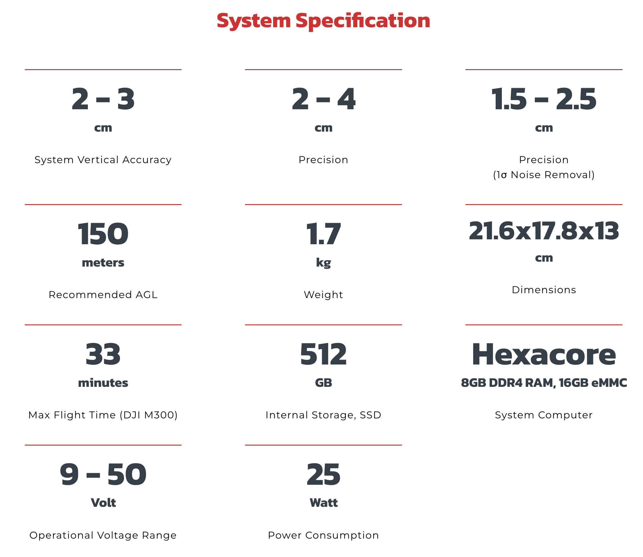
The GEN-II’s powerful on-board computing module allows for real-time point cloud visualization (for quality control and fast decision making) and supports integration of external sensing modules, letting users synchronize additional cameras, LiDAR, or input aiding data from various sensors. This makes it a highly customizable and versatile plug-and-play hardware package, ideal for end-users and engineering firms. Some of the system specifications are shown below in Figure 3.
2. Mobile Mapping Study Description
To demonstrate the capabilities of the system, we organized a mission in a mobile configuration. Most suppliers sell results and performance specifications that in reality turn out to be only ideal-conditions which are almost never replicable for the end-user. Inertial Labs prides itself in not only making quality products but being a trustworthy partner that offers integrity and honesty.
A typical mobile mapping mission includes the following as an operating procedure for data acquisition:
- 30 second to one-minute static alignment in ideal GNSS conditions (open sky);
- 5 minutes of driving in ideal GNSS conditions where observable changes in heading, position, pitch and roll are experienced – prior to driving into mission area;
- User proceeds to area of interest for mapping. This duration of time varies based on project. Depending on conditions of GNSS, consider including segments of coverage in areas of high-quality GNSS to ensure positional accuracy throughout the dataset.
- 5 minutes of driving in ideal GNSS conditions where observable changes in heading, position, pitch and roll are experienced – after driving out of mission area;
- 30 second to one-minute static alignment in ideal GNSS conditions (open sky);
For this test, we spent only a few moments in quality GNSS coverage before proceeding into areas with dense tree cover. This was done intentionally to demonstrate the power of a less-than-optimal workflow to highlight the capabilities of the Kernel-210 Inertial Labs IMU with a dual antenna GNSS receiver inside the RESEPI GEN-II system.
Below is a brief description of the test that was performed:
Location: Paeonian Springs, Virginia, USA.
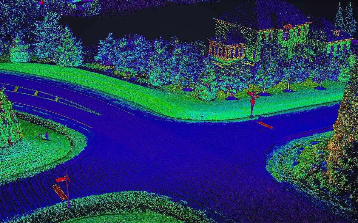
Terrain type: Paeonian Springs, Virginia, is characterized by gently rolling countryside, representing a rural-suburban transition area within the broader Virginia Hunt Country. It features a mix of wooded areas and open farmlands, as shown in in Figure 4.
Land Features: The presence of tall trees with dense crowns (Figure 5) coupled with open skies.
Mission Purpose: To showcase the performance of RESEPI GEN-II as a mobile mapping solution when standard operating procedures are not followed and in effect demonstrate to customers what performance can be achieved even in less-than-ideal conditions.


Equipment used: For this project, we deployed a standard set of RESEPI available equipment as follows:
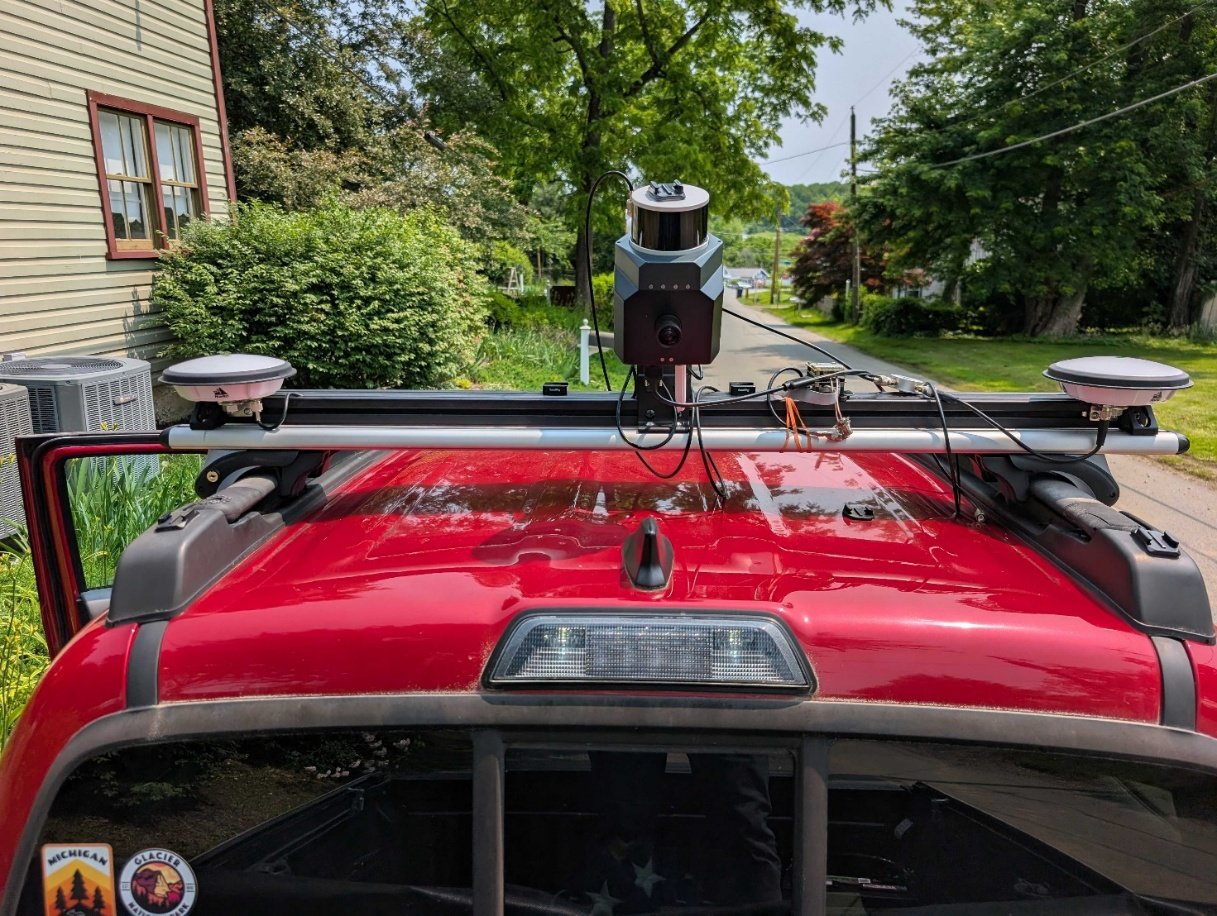
Mobile Platform: A pickup truck served as the mobile platform, specially adapted for the stable mounting of geospatial equipment.
Remote Sensing System (Payload): The core data acquisition system was the RESEPI GEN-II with XT-32M2X LiDAR. This advanced LiDAR configuration, featuring the lighter XT-32M2X scanner with an extended detection range, was crucial for capturing high-accuracy and dense point clouds, vital for detailed mapping requirements.
Navigation Equipment: The RESEPI GEN-II system integrates Inertial Labs’ Dual Antenna Inertial Navigation System (INS-D), which includes a Tactical Grade Kernel-210 IMU and a dual antenna NovAtel OEM7720 GNSS receiver.
Dual-Antenna Mobile Mount: To optimize the performance of the dual-antenna INS on the previously mentioned pickup truck, a customized mount was installed (Figure 6). This ensured precise spatial placement and stability for the GNSS antennas. NovAtel Vexxis 802L multiband GNSS antennas were used.
Software: Inertial Labs’ PCMasterPro and LiDAR360 from Green Valley International.
Ground Control Points: Both control point and check points were gathered using differentially processed base data from an Emlid RS2+ recording static sessions with a minimum of 15 minutes each logged at a data rate of 20Hz.
3. Data Capture for Study in PCMasterPro
Using Real Time Streaming into PCMasterPro as Quality Control Tool
An indispensable feature of RESEPI GEN-II is the support of real-time data capture and transmission. Previously, the user organized a mission, then processed the data after. This would have been the users’ first opportunity to get a look at the point cloud. Although many tools exist to verify successful operation of the payload, nothing beats being able to look at a 3D representation of the environment you are scanning in real time to know for certain that capture is happening as expected. The ability to track data recording in real time will save the user a lot of time, and here’s why:
- Coverage assessment: You can see immediately, whether you’ve covered all the area you need to cover, exposing if there are any data gaps or “holes” in the point cloud that may require revisiting.
- Save time and resources: Instead of collecting data all day and then finding errors only after uploading and post-processing in the office, you can fix them on the spot before leaving the job site. This significantly reduces project turnaround time and reduces the cost due to repeat missions.
- On-site decision making: If you see that the data quality is excellent, you can complete the mission earlier or, conversely, decide it’s worth collecting more data in a certain area because time permits.
- Confidence in the outcome: When you see real-time data, you can be confident that the system is working correctly and collecting exactly what you need.
- Minimize risks: Continuous monitoring helps you avoid costly errors that can occur due to misconfigured equipment or external factors.
- Quickly detect anomalies: Unusual readings or abnormalities are immediately apparent, allowing you to immediately investigate the cause.
In essence, real-time data recording and visualizing is like an airplane dashboard for a pilot: it gives you all the information you need right now so you can make informed decisions, avoid errors, and do your job as efficiently as possible.
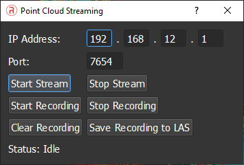
In PCMasterPro, to monitor and visualize real-time point clouds, simply click on the menu “Data Streaming” -> “Settings”. The window shown on the Figure 7.
Using Fixed versus Estimated Lever Arms versus for Optimal Accuracy and Precision
In our previous articles, we have repeatedly mentioned that PCMasterPro uses NovAtel Inertial Explorer (IE) for post-processing GNSS+IMU data. But we have not previously considered in detail the features of its operation, particularly the Lever Arm Definition. PCMasterPro (thanks to IE) has functionality that allows you to estimate (calibrate) levers – that is, the displacement vector between the GNSS antenna(s) and the IMU center. This procedure is called lever arm estimation.
How it works:
- During post-processing (Forward/Reverse/Combined), IE analyzes INS and GNSS data using the differences between the expected and measured trajectory.
- Based on the dynamics of movement (especially in 3D), IE can estimate the antenna displacement vector, minimizing errors between the INS and GNSS position.
Ideal conditions for a good estimate:
- There should be a variety of movements (not only a straight line): turns, tilts, accelerations, even static conditions for biases to be estimated at beginning and end.
- Antenna(s) are placed in locations where they are not hidden underneath structures that block line of sight with satellites.
- During the data capture, it is important for there to be quality GNSS coverage during the entire operation. Low exposure of satellites (tunnels, narrow canyons) or satellite visibility from low elevation angles result in poor estimates of antenna positions.
PCMasterPro assumes that the GNSS antenna(s) are fixed relative to the IMU. If it is moving (e.g. on a flexible bracket), the result will be inaccurate. If all conditions are met, the software will automatically estimate the offset to within an estimate accuracy of 1 mm.
But there is another, more reliable approach especially for mobile environments where areas with poor satellite coverage may exist and be common. If the offsets are already known whether by measurement or by CAD drawing, you can process manually assigning these as the desired values to use during point cloud creation. In cases of poor GNSS environments you will always end up with a more reliable and accurate solution if you do this, and here’s why:
- Maximum reliability: if measured accurately, it is “ground truth”, independent of the algorithm.
- More predictable result: there is no risk that the program will make a mistake due to lack of maneuvers or noise.
- Less dependent on the trajectory: even if the trajectory is simple or straight, the values will still be correct.
Of course, not everyone will be able to measure an arm manually with an accuracy of 1 mm without having special equipment. Therefore, we have given recommendations on how to get the best results in PCMasterPro by combining automatic estimation and manual input of lever arms, as follows:
- If in environment with perfect conditions:
- Use dual antenna processing, sampling rate of differential solution = 20Hz, Lever Arm Refinement = auto;
- If in environment with non-perfect conditions:
- Use dual antenna processing, sampling rate of differential solution = 1Hz, Lever Arm Refinement = off;
- Forced lever arm values must be KNOWN. For best results, perform initial drive test in perfect environment, use refine lever arm features to determine the exact lever arm, and then use these values to manual input lever arm in environments that are not good.
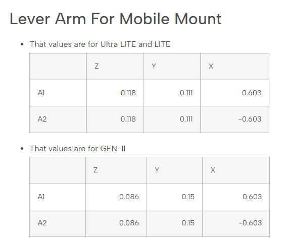
- Alternatively, if using our mobile mount hardware, we provide exact lever arm values computed from CAD software (see below).
Using our proprietary mount (Figure 8), the user does not need to perform an initial drive test because we have already computed results perfectly from our design software. The user simply specifies the offsets in PCMasterPro and the software does the rest for you.
4. Dual Antenna Pre-Processing in PCMasterPro and Point Cloud Creation
Returning to our mission, after collecting the data, we processed it in our proprietary PCMasterPro software. The processing procedure is very simple and does not require any significant competencies. Below we provide detailed instructions on how to process dual-antenna GNSS projects in PCMasterPro:
- Copy the raw project data to your computer.
- Open them by double-clicking on “ppk.pcmp” or directly in PCMasterPro via the menu “File” -> “Open Project”.
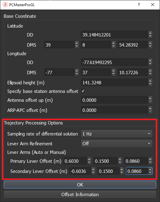
- The program will unpack the archives and display a window with data entry for the base station and antenna offsets, as shown in Figure 9. Note that we selected the 1Hz frequency and manually set the antenna offsets that were shown in Figure 8. This was done intentionally because the GNSS quality in the environment driven was not perfect and prone to error to do poor satellite visibility on tree-covered rural roads.
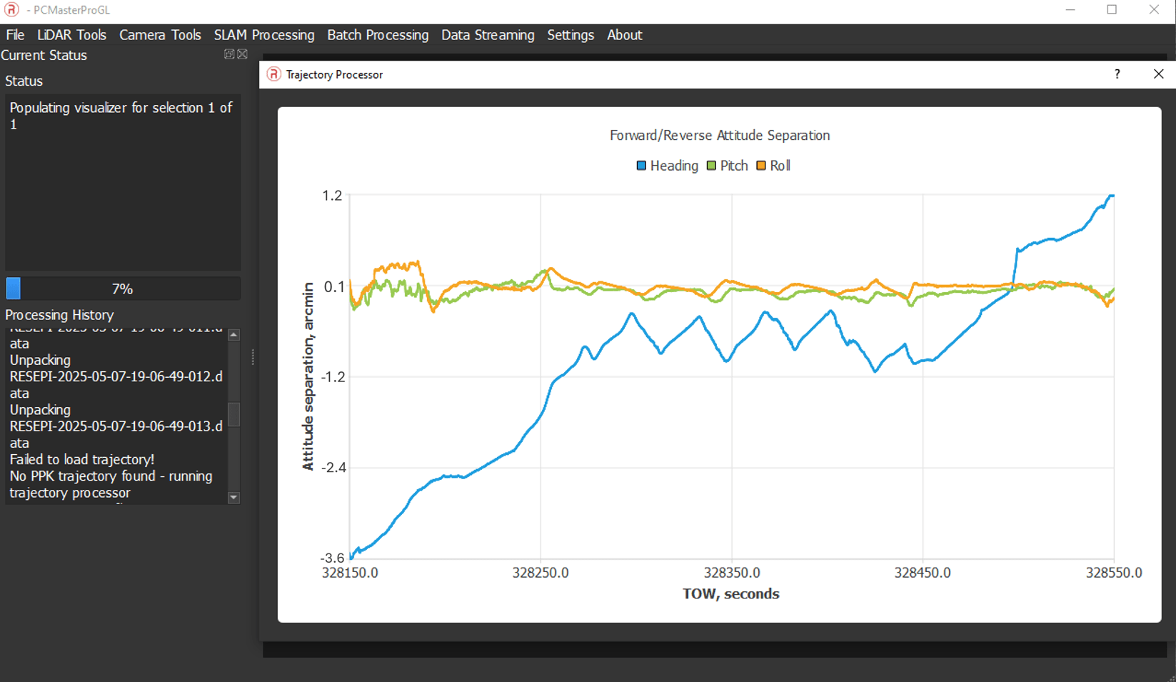
- After entering the parameters, click “OK”. This will start the processing, which no longer requires user intervention (Figure 10)
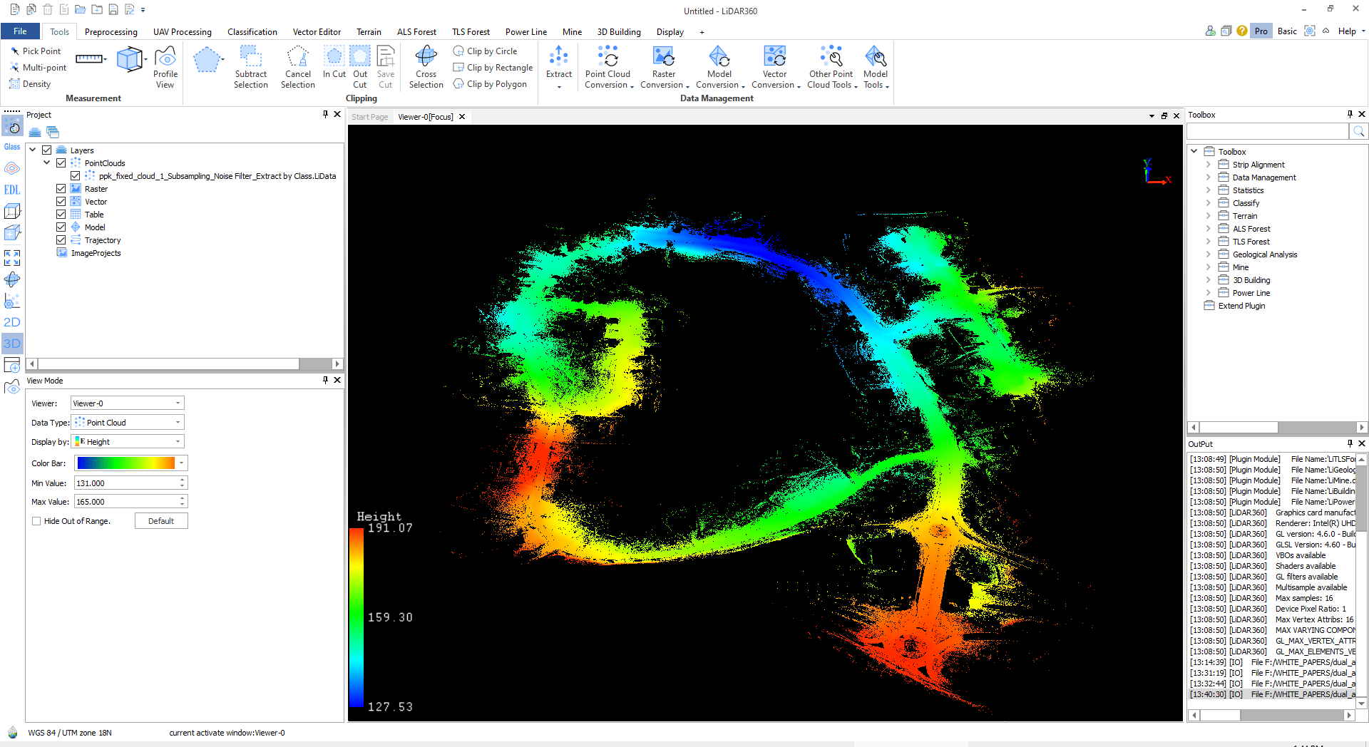
- After completing the data processing, we obtained the point cloud shown in Figure 11.
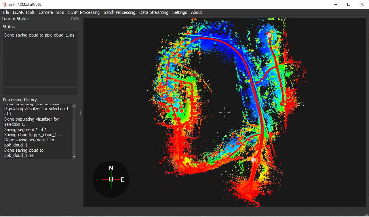
- Select the portions of the path you would like to output the point cloud for.
- We now exported this point cloud for further processing to follow a typical MMS workflow in LIDAR360 from GreenValley [4].
Next, we look at the post-processing procedure for a MMS workflow and resulting accuracy assessments in LiDAR360.
5. MMS Post-Processing in LiDAR360 for Alignment and Adjustment with Ground Control
Due to the complex nature of GNSS conditions associated with mobile mapping, most state and local entities encourage and even require the use of ground control for not only accuracy assessment but correction. This helps ensure reliability and proper alignment with local defined geographic landmarks. LiDAR360 from GreenValley contains some helpful tools where we will show what accuracy is achieved in a less-than-optimal environment. In this section, we will walk through a typical MMS workflow to assess accuracy of classified ground points. First, we begin by importing the point cloud. In LiDAR360, this can be done in several ways:
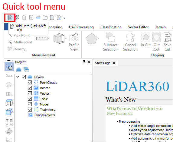
- Use the Quick Access menu in the upper-left corner, as shown in Figure 12a.
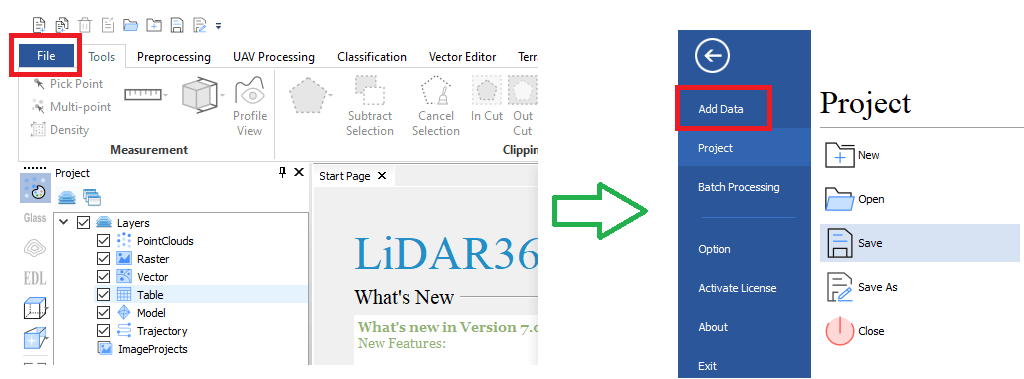
- As shown in Figure 12b, click on the “File” button and then click on “Add Data” in the window that opens.
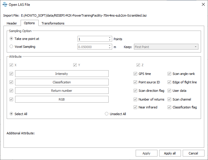
A dialogue box will pop up to specify the path to the .las (.laz) file.
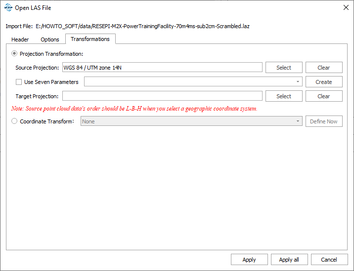
After selecting the file, the program will display the header information of the .las (.laz) file in the window shown in Figure 13 (a, b, c).

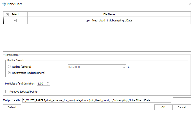
The standard next step is to filter the point cloud for noise. To do this, click “Other Point Cloud Tools” -> “Noise Filter” on the “Tools” tab. For the demonstration we also used default settings, as shown in Figure 16. But in your case, you may need to tweak the parameters to achieve the best results.
Once the filtering is complete, go to the “Classification” tab and click on “Classify Ground Points”. The window shown in Figure 17 will open.

We also used the default settings, but the user should adjust them as needed to get the best results. Then, select the preset according to the type of terrain, in our case it is a slightly hilly terrain with vegetation. After classification we return to the “Tools” panel, click ‘Extract’ -> “Extract By Class” and specify the class “Ground”. Then we will work only with the ground-point cloud. The result is shown in Figure 18.
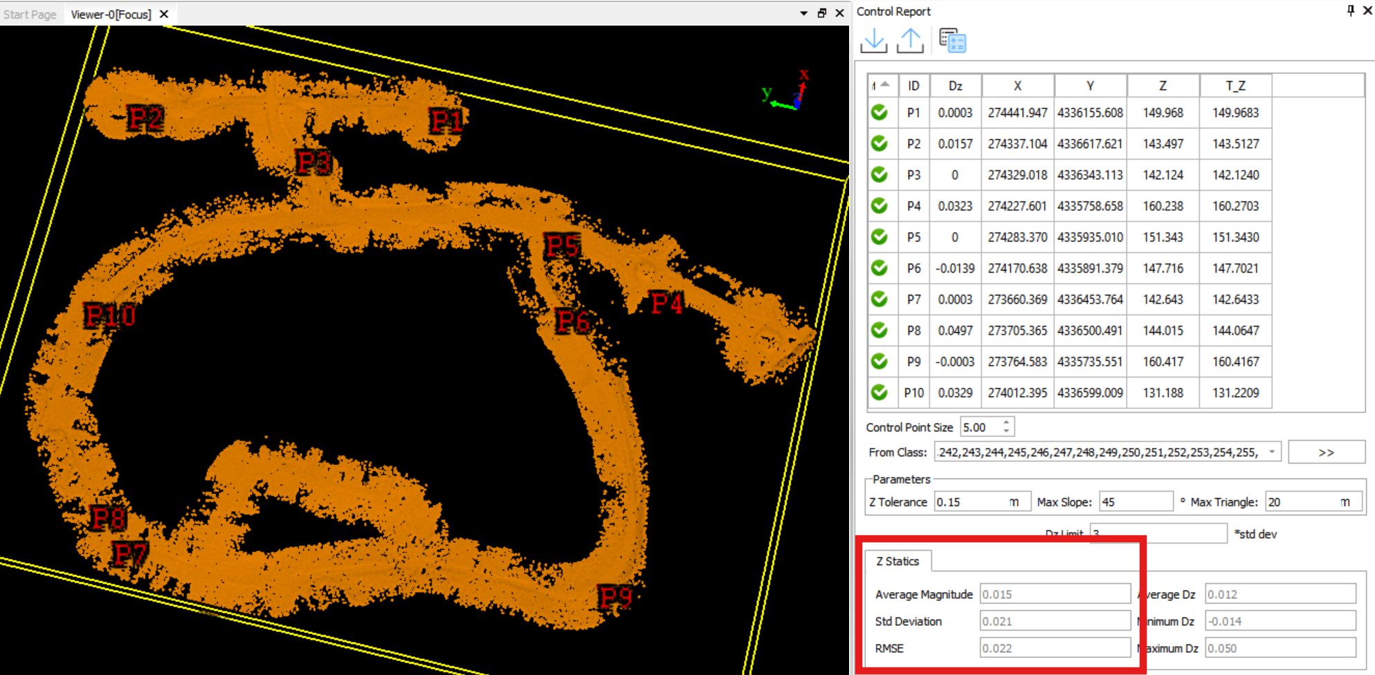
Next, control points were brought into the project. On the “Preprocessing” tab click on “3D Control Point Report”. In the opened window select “Check Type” – “Elevation” and click “OK”. Click on the icon to open a file with GCPs. The point cloud was de-biased with the control points and then analyzed for errors. After importing and adjusting the points to align them to the coordinate system of the project, set the required fields according to the order of data in the file and click run “Control Point Report”. Results are shown below in Figure 19.

It is important to note P7 stands out as an outlier from the dataset that is being analyzed. Multi-constellation/frequency differential GNSS solutions, especially with baselines like ours of less than a kilometer have well known accuracies of sub 3cm. For our control points to have any alignment error of -7.2cm is noteworthy. This point typically would be collected again or analyzed further, however one of the main purposes of this case study is to highlight the powerful alignment tools within LiDAR360. For this purpose, it was kept and used for the duration of the case study.
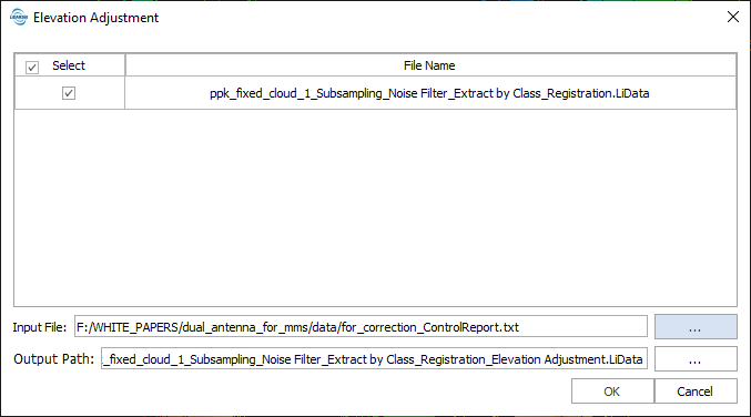
With all points considered, the average magnitude is 3.1 cm and the RMSE error is 3.7 cm. These results alone are not bad results, but in a traditional MMS workflow the use of control points to correct the data are often required, and will see what happens when we do the same. For this we will use the utility “Elevation Adjustment”. To use this utility, we need to export “Control Point Report”. For correction we will use 5 points out of 10, and in our case, we have chosen 1, 3, 5, 7, 9.
Now we will correct the error using the automatic alignment in the “Preprocessing” -> “Transformations” -> “Elevation Adjustment” tab. In the window that opens, specify the path to our new report file, as shown in Figure 20.
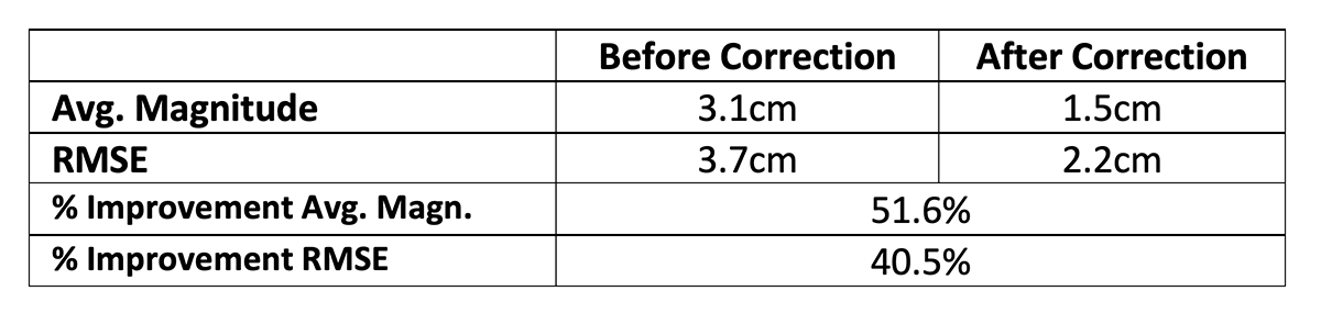
As you can see, the result is an average magnitude = 1.5 cm, and RMSE = 2.2 cm. Excellent accuracy in difficult GNSS signal conditions, and very good error compensation.
By leveraging our cutting-edge hardware, including the RESEPI GEN-II with XT-32M2X LiDAR and its integrated Inertial Labs’ Dual Antenna INS-D, combined with sophisticated processing software, we achieved remarkable precision in our data. A summary of the results can be seen below in Figure 22.
This level of accuracy, was attained without incurring excessive labor costs or requiring extensive manual intervention, highlights our commitment to best-in-class solutions and translates directly into superior, efficient, and highly reliable results for our clients.
6. Conclusion and Discussion
This study demonstrated the practical performance and reliability of the RESEPI GEN-II with XT-32M2X LiDAR, equipped with the Inertial Labs Dual Antenna INS-D, in a real-world mobile mapping scenario under less-than-ideal GNSS conditions. The results clearly highlight the advantages of a dual-antenna integration, robust IMU performance, and intelligent software processing within PCMasterPro and LiDAR360.
Despite intentionally minimizing ideal GNSS initialization and exposing the system to dense vegetation and intermittent satellite visibility, the system achieved highly accurate and consistent results. Before ground control alignment, the system produced an average magnitude error of 3.1 cm and an RMSE of 3.7 cm. Following elevation adjustment and automated correction within LiDAR360, accuracies improved significantly to 1.5 cm / 2.2 cm. These results represent a 52% improvement in average magnitude and over 40% improvement in RMSE, highlighting the effectiveness of the integrated hardware–software workflow.
Governing bodies such as: USGS, ASPRS, FHWA, DOT, lay out the requirements by which most federal, state, and project-specific jobs are defined by. These requirements include many things specifying vertical accuracy, horizontal accuracy, control spacing for ground points, and many other operational procedures to ensure consistency and accuracy across the many public and private entities that utilize such standards. Most mobile projects require a vertical accuracy of less than 5cm RMSE and a horizontal accuracy that is twice that, being less than 10cm RMSE. California and New York have some of the tightest requirements where many jobs will have vertical accuracy requirements of even 2cm or less. For these jobs control spacings are typically tight (every few hundred meters) where corrections are not just expected, but required, to ensure any and all drift or GNSS related errors are corrected for.
The RESEPI system, as shown from this case study, even with a less-than-optimal workflow demonstrates capabilities that directly translate into practical solutions for problem spaces of: corridor mapping, bridge and pavement inspections, infrastructure management and even engineering design work.
In conclusion, this case study validates the RESEPI GEN-II platform as a highly capable and dependable mobile mapping solution that performs exceptionally well even outside ideal conditions. The combined use of dual-antenna GNSS, a tactical-grade IMU, and advanced software integration ensures centimeter-level precision, reduced field time, and streamlined project workflows. These results establish a strong foundation for future deployments in urban, forested, and otherwise GNSS-challenging environments—confirming Inertial Labs’ commitment to providing reliable, accurate, and field-ready geospatial solutions.
References
[1] “Deep Dive into RESEPI Accurate Data.” Inertial Labs, 25 Mar. 2025. Accessed 28 July 2025.
[2] “RESEPI GEN-II M2X-ILX.” RESEPI, 7 Mar. 2025.
[3] “Real Time Point Cloud Streaming.” RESEPI, 7 July 2025. Accessed 28 July 2025.
[4] “LiDAR360 Point Cloud & Images Post-Processing and Industry Applications Software – GreenValley International.” Greenvalleyintl.com, 2022.