Overview
Why do some LiDAR mapping systems produce better data than others? While many factors (Figure 1) can affect output point cloud quality, high-performance system hardware is one key factor and the foundation of the rest. This article profoundly delves into this subject and explains why the Inertial Labs INS (Inertial Navigation System) enables RESEPI (Remote Sensing Payload Instrument) to outperform competitors in the same LiDAR payload class. We discuss key features that make this system ideal for high-precision applications such as LiDAR surveys, mapping, and geodetic measurements. Sensor innovations that ensure stability and accuracy in the most demanding environments are reviewed, along with features that avoid calibration issues and accuracy reduction.

Figure 1. Factors that affect the accuracy of the point cloud.
Special attention is given to the high level of integration with other systems and filters, which significantly improves performance and data quality. In this article, you will learn why Inertial Labs’ INS is not just a solution but a true revolution in accuracy and reliability for your business.
Here are the sections that will be covered: “When every centimeter counts: the role of INS in LiDAR data accuracy,” Error Source: Why doesn’t the Kalman filter always solve the problem?”, “Why Inertial Labs’ INS outperforms the competition,” and “PPK: The key to LiDAR survey accuracy.” The conclusion will summarize the benefits of using Inertial Labs’ INS in LiDAR payloads.
Modern Applications Need Accurate LiDAR Mapping Data
Modern infrastructure and development projects require the creation of detailed and accurate terrain models, where minor errors can have significant consequences. In the construction industry, high-precision point clouds monitor progress, plan and control heavy equipment, and verify that finished projects meet design standards. When inspecting bridges, dams, or powerlines, high accuracy is often needed even in GNSS-denied environments (e.g., in urban areas or under dense vegetation). Digital twins are becoming more widely adopted in many industries. At the core of these solutions is a requirement for measuring precise position and orientation to ensure that each map element correctly aligns with the other, most often in a global coordinate system. All these applications need sensor-fusion mapping technologies with high positioning and orientation accuracy, which rely on a high-precision INS solution [2].
The development of INS technologies, such as those from Inertial Labs, not only helps solve these challenges but also sets new standards for accuracy and efficiency by making technologies that were once inaccessible to many industries within reach, driving cost-effective innovations. Inertial Labs INS integrated with RESEPI offers a unique combination of accuracy, functionality, and affordability [3].
Better INS Enables More Accurate LiDAR Mapping Data
For a navigation-based LiDAR mapping solution, the INS is a core system component. To create a georeferenced point cloud, the solution first needs to resolve the mission trajectory (its system positions and orientations at every timestamp), then project LiDAR points at each epoch of the trajectory using the LiDAR’s collected distance and scanning angle for each return. In this context, the performance of the INS becomes critical for the accuracy of the output point cloud because it offers the system the capability to measure global position and orientation, which is the reference from which the LiDAR points are projected. LiDAR can provide point clouds of very high density. Still, without accurate information about the system sources’ position and orientation in space, this data will be challenging to interpret (or unusable) because even minor errors in angular and linear measurements can lead to propagated errors over the entire project. For example, if the mistake along one of the x/y/z axes is 0.1 degrees, then at 50 meters, the error in determining the coordinate will be off by about 17.5 cm. However, with an error of 0.01 degrees and the same distance, the mistake of selecting the coordinate will be reduced to 1.75 cm. In short, precision and accuracy matter significantly when errors can compound.
In addition, the high accuracy of the INS in combination with LiDAR allows more efficient implementation of techniques such as LiDAR-based SLAM (Simultaneous Localization and Mapping), where one the most important contributors to the accuracy of the SLAM solution at each epoch is the motion model that can be derived from the data produced by the INS which is used to correct the map and trajectory estimation [10]. In such systems, an INS can provide data with a low error rate so that the system can better track changes in position and orientation. To accomplish this, systems typically use integrated solutions where data from INS and LiDAR are processed together through a Kalman filter. For such advanced systems, the accuracy of the INS data remains a basis for the correct and reliable operation of the SLAM algorithm without the risk of failure or instability introduced where LiDAR features or frame-to-frame motion render the algorithm unable to estimate its current state.
Thus, INS accuracy and stability become key to ensuring accuracy in LiDAR systems of various kinds, especially when integrated with other sensors and when using complex algorithms such as SLAM. Proper calibration and error minimization in INS sensors will maximize the use of LiDAR data, providing high-quality and accurate results in applications ranging from autonomous vehicles to geodetic surveys.
What Affects the Accuracy of Position and Orientation Determination?
At the “heart” of an inertial navigation system are Gyroscopes and Accelerometers [4]. Gyroscopes and Accelerometers form the basis of an Inertial Measurement Unit (IMU), providing data for calculating an object’s orientation, velocity, and position. Gyroscopes measure angular velocity around the three axes (X, Y, Z) using the effects of inertia, such as the Coriolis effect in MEMS gyroscopes, Figure 2 [5]. This data allows the current orientation of an object to be determined through the integration of angular velocities. However, gyroscopes have a bias and are also subject to systematic drift, which leads to an accumulation of angular error, as shown in Figure 3. Also, let’s not forget about random noise causing additional measurement errors. In addition, their sensitivity or errors can vary with temperature, which requires correction algorithms [6].

Figure 2. IMU designation.
Accelerometers, in turn, measure linear acceleration in three axes, capturing changes in object motion linearly. They can determine orientation from gravitational acceleration under static conditions and even calculate an object’s local position through the double integration of accelerations. However, accelerometers are also susceptible to zero drift. Random noise and vibrations exacerbate this problem, reducing the accuracy of measurements under dynamic conditions.

Figure 3. Gyroscope bias and drift.
To compensate for these errors, filters and algorithms, such as the Kalman filter, combine IMU data with external sources (e.g., GNSS or magnetometer), smoothing noise, and correcting for accumulated errors [6]. Many filters attempt to use the best of each available sensing component offering, using the other to correct for its faults.
However, even the most advanced algorithms cannot eliminate systematic drift or error, making sensor quality, zero drift minimization, and stability of sensor performance critical for high-precision IMU operation.
Why Can’t the Kalman Filter Fully Compensate for Errors?
The Kalman filter is a powerful tool for processing sensor data and improving the accuracy of system state estimation, but its ability to compensate for IMU errors has limitations. The main problem is that the Kalman filter assumes a linear model of the system dynamics and the best knowledge of the statistical properties of the noise. In reality, many IMU errors, such as gyro and accelerometer drift, are nonlinear and time-varying, making it difficult to compensate for them entirely using a standard Kalman filter. In addition, the Kalman filter requires accurate noise models. Still, in the case of IMUs, noise often depends on multiple factors such as temperature, vibration, or electromagnetic interference, making it challenging to model and account for in the filter.
The following methods are commonly used to compensate for such errors:
- Long-term Calibration. Sensors are tested in a laboratory environment to determine the static zero offset. The calibration parameters are stored in the microcontroller. This approach is used in most commercial IMUs.
- Baseline Averaging. The average of the steady-state readings is determined and then subtracted from the current data.
- Thermal Compensation. Temperature-dependent offset models are created based on laboratory measurements. Linear approximation, polynomial approximation, or exponential models are often used.
- Temperature Sensors. Built-in temperature sensors record the current temperature, and the algorithm adjusts it based on the temperature model.
These are basic and commonly used methods that can be integrated into the Kalman filter, but in general, the filter itself cannot correct all the IMU errors, as shown in Figure 4.

Figure 4. The result of the Kalman filter.
The Kalman filter is described by two main equations: prediction equations and update equations. The covariance matrices ![]() and
and ![]() play a key role in these equations, determining how the filter accounts for system dynamics and measurement uncertainty.
play a key role in these equations, determining how the filter accounts for system dynamics and measurement uncertainty.
Prediction Equations estimate the state and error covariance based on the system model (4):
 (4)
(4)
where ![]() is the predicted state of the system,
is the predicted state of the system, ![]() is the state transition matrix (dynamic model);
is the state transition matrix (dynamic model); ![]() is the control matrix,
is the control matrix, ![]() is the control vector,
is the control vector, ![]() is the expected error covariance,
is the expected error covariance, ![]() and is the process noise covariance matrix.
and is the process noise covariance matrix.
A larger ![]() value indicates less trust in the model and more reliance on measurements. A smaller
value indicates less trust in the model and more reliance on measurements. A smaller ![]() increase in trust in the predicted dynamics.
increase in trust in the predicted dynamics.
Update Equations to correct the prediction using new measurements (5):
 (5)
(5)
where ![]() is the Kalman gain (weighting coefficients);
is the Kalman gain (weighting coefficients); ![]() is the measurement vector;
is the measurement vector; ![]() is the measurement matrix (links the state to the measurements), and
is the measurement matrix (links the state to the measurements), and ![]() is the measurement noise covariance matrix.
is the measurement noise covariance matrix.
A larger ![]() indicates less trust in the measurements. A smaller
indicates less trust in the measurements. A smaller![]() increases the influence of measurements on the final state.
increases the influence of measurements on the final state.
To improve the performance of the Kalman filter, several key approaches can be applied:
- First, carefully tuning the process and measurement noise is essential. Noise parameters Q and R significantly affect the accuracy of the filter. Improperly chosen values can cause the filter to either trust the measurements too much (in the case of too low a value for R) or not account for them properly (if R is too large). Adaptive methods are often used for more accurate modeling to adjust to these noises as the filter performs dynamically.
- Second, in the case of using a Kalman filter for nonlinear systems, it may be necessary to use an extended Kalman filter (EKF) that approximates the nonlinearities using linear approximations. This requires appropriately developing nonlinear models for states and measurements and the computation of their Jacobians. It is vital to ensure that these models accurately reflect the fundamental processes of the system so that the filter can update its estimates correctly.
- A third important point is the proper initialization of the initial conditions. If the initial values of the condition or covariance are chosen too far from the fundamental values, the filter may take a long time to converge or sometimes not converge. Using more accurate estimates of initial states or performing pre-filtering for correct initialization is recommended.
- Combined methods can also be used, such as a Kalman filter using multivariate data or combining the Kalman filter with other methods, such as particle filtering, to improve robustness and accuracy in the face of high noise or dynamic changes in the system. It is also worth considering implementing models to account for sensor drift, such as gyroscopes and accelerometers. This can significantly improve the long-term accuracy of the filter if drift is a significant factor in the system.
Thus, to improve the efficiency of the Kalman filter, it is essential not only to tune the filter parameters properly but also to deeply understand the dynamics of the system the filter is working with and to pay attention to possible improvements to the models and computational methods.
Using Multidimensional Data or What is Sensor Fusion
Using external data from different sensors (Sensor Fusion) can significantly improve the accuracy and robustness of the Kalman filter, especially in complex applications such as positioning and navigation systems [7]. Incorporating additional sensors into the filtering process can compensate for inefficiencies and errors that may arise due to noise or limitations of individual sensors.
The incorporation of data from external sensors such as GPS, magnetometers, or barometers can compensate for gyro drift and reduce the accumulation of errors in integrated measurements, especially in long-duration measurements. In addition, dynamic environmental data, such as data from a camera, can further improve positioning in complex or poorly controlled environments, such as urban canyons or enclosed spaces [8].
In addition, using external data also helps make the filter more resilient to abnormal situations or sensor malfunctions. For example, suppose one of the sensors fails or starts giving false data. In that case, the filter can automatically adapt and rely on other, more reliable sources of information, minimizing the effect of the malfunction. For example, this could be GNSS signal spoofing (spoofing) or jamming, so the algorithm will not use GNSS data but rely on odometer and/or barometer data [9].
Thus, external data can significantly improve the accuracy and robustness of the Kalman filter, providing more robust and adaptive solutions, especially under uncertainty or with limited internal measurements.
Why Inertial Labs’ INS Outperforms the Competition
RESEPI utilizes a variation of the IMU Kernel-210 with high-accuracy gyroscopes and accelerometers. We compared its characteristics with commonly used competitor solutions and provided an understanding of where they sit when comparing prices. The comparison results are shown in Table 1. Let’s understand what these parameters mean and how they affect accuracy.

Table 1. Comparison of IMU Kernel-210 characteristics with competitors.
The declared datasheet values are often measured under ideal laboratory conditions. To this end, manufacturers carry out special calibration procedures to determine the errors of their IMUs. The values provided in Table 1 are residual errors after thermal calibration. The sensors are calibrated over a wide temperature range—in this case, from –40 to 85 degrees Celsius—to ensure functionality in real-world conditions.
Gyro Bias repeatability. The “bias” of a gyroscope is the angular velocity value that the gyroscope indicates when it is stationary. Ideally, these values should be zero, but in real devices, they may have a nonzero value at rest due to sensor peculiarities.
“Repeatability” shows how consistently this offset (within the specified temperature range) occurs every time the gyroscope is turned on and off. Good repeatability means the bias will be approximately the same at each startup; poor repeatability implies that the bias may vary noticeably from one startup to the next. As can be seen, the KERNEL-210 has the lowest value, so temperature changes will affect its accuracy much less compared to competitors, whose bias is over eight times larger.
Gyro bias in-run stability. “In-run stability” indicates how much the gyroscope’s bias changes during operation. Even if the bias is well-calibrated at startup, it may “drift” or change slowly over time. High stability means that the bias remains almost constant over long periods of operation.
Gyro Scale Factor error. “Scale Factor error” is the deviation of the scale factor from its ideal value. This means the gyroscope may output slightly different values for the same actual angular velocity due to the scale factor error.
ARW. “Angular Random Walk” is a characteristic that describes the random noise in the gyroscope’s output signal. It measures how the integrated angle drifts randomly due to this noise. Even without drift and zero scale factor error, ARW will introduce random and unpredictable errors in the orientation estimation, accumulating over time following a random walk process (roughly proportional to the square root of time).
Since we have clarified the differences and the importance of these parameters, let’s consider their impact on orientation accuracy.
For assessing the accuracy of such extensive and complex systems as an INS, it is common to simulate the system’s performance under various conditions (stationary base, rocking, accelerated motion, etc.). However, for a simple error estimation, one can use the simplified formulas of the gyroscope signal model [10].
For gyroscopes, the impact of drift on the accuracy of angle measurements with a stationary base can be estimated using equation (1). In this case, we assume that the drift is constant.
 (1)
(1)
where ![]() is the gyroscope drift, and
is the gyroscope drift, and ![]() is the operating time without external correction.
is the operating time without external correction.
The impact of noise is expressed by equation (2):
 (2)
(2)
where ![]() is the gyroscope noise (or Angular Random Walk)
is the gyroscope noise (or Angular Random Walk) ![]() ?
?
The scale factor error is expressed by equation (3):
 (3)
(3)
where ![]() is the scale factor error
is the scale factor error ![]() , is the angular speed
, is the angular speed ![]()
To determine which parameters have the most significant influence, we substitute the values from Table 1 for the KERNEL-210 and calculate the errors for each component. In doing so, we set the time t = 60 sec and assume ![]() is operating within its’ worst-case scenario, i.e., as the sum of both biases: Gyro Bias repeatability and Gyro bias in-run stability. We will also assume that the angular velocity
is operating within its’ worst-case scenario, i.e., as the sum of both biases: Gyro Bias repeatability and Gyro bias in-run stability. We will also assume that the angular velocity ![]() = 3 deg/s. The result of the angular measurement accuracy calculation is shown in Table 2.
= 3 deg/s. The result of the angular measurement accuracy calculation is shown in Table 2.

Table 2. Angle measurement accuracy calculation result.
As can be seen from the results, the most significant sources of error are bias and scale factor error.
By integrating the acceleration (accelerometer signal) twice, we obtain the displacement value, or, in other words, the change in position. The effect of the zero offset can be estimated using the formula (4) [11]:
 (4)
(4)
where ![]() is the accelerometer bias
is the accelerometer bias ![]() .
.
The effect of the scale factor shift is estimated using the formula (5):
 (5)
(5)
where ![]() is the scale factor error
is the scale factor error ![]() , and is the distance traveled
, and is the distance traveled ![]() .
.
The error caused by VRW noise is expressed by the following formula (6):
 (6)
(6)
where ![]() is accelerometer noise (or Velocity Random Walk)
is accelerometer noise (or Velocity Random Walk)  .
.
As with gyroscopes, we also substitute the values from Table 1 for the KERNEL-210 and calculate the errors for each component. In doing so, we set the time t = 60 sec and assume ![]() is operating within its’ worst-case scenario, i.e., as the sum of both biases: Accel Bias repeatability and Accel bias in-run stability. We will also assume that the distance
is operating within its’ worst-case scenario, i.e., as the sum of both biases: Accel Bias repeatability and Accel bias in-run stability. We will also assume that the distance ![]() = 1000 m. The result of the coordinate accuracy calculation is shown in Table 3.
= 1000 m. The result of the coordinate accuracy calculation is shown in Table 3.

Table 3. Angle measurement accuracy calculation result.
As can be seen from the results, the most significant sources of error are bias and scale factor error.
To demonstrate the superiority of the KERNEL-210, we calculated the errors under the same conditions using the specifications of competing solutions from Table 1. The result is shown in Table 4.

Table 4. Result of IMU KERNEL-210 comparison.
The outcome demonstrates the advantages of the KERNEL-210 IMU compared to its competitors. Despite being somewhat inferior in noise characteristics compared to the competitive landscape, some performance characteristics come at a significant cost difference. The gyroscopes in KERNEL-210 achieve high accuracy due to superior performance in parameters that are far more important than noise. As a result, when integrated into systems like RESEPI, users can expect to see point clouds with reliable accuracy when surveying applications.
The Kernel-210 IMU is designed to operate in harsh environmental conditions and, as mentioned, has a high reliability rating. MTBF (GM @+65degC, operational) is 100000 hours. Long service life and stable operation reduce maintenance and replacement costs. No one wants to interrupt work and face losses due to the need for IMU maintenance or calibration.
Additionally, our IMU provides a high data update rate of 2000 Hz. A higher frequency allows for faster movements to be tracked.
We conducted real-world tests and scanned a section of territory with the RESEPI XT32 at a 100 km/h speed, as shown in Figure 5. The flight altitude was about 50 m, the recommended AGL for this model, and was used on a manned aircraft.

Figure 5. RESEPI velocity chart during operation.
The point cloud obtained in this way is shown in Figures 6 and 7. As you can see, the relative accuracy is just over 4 cm. This explanation aims to showcase the benefit of higher update rates and their impact on data quality. Although fully capable, as seen in other papers, for use on VTOL aircraft and multi-rotor UAVs, RESEPI is not limited to these platforms and can be used on larger vehicles, even manned aircraft.

Figure 6. General view of the point cloud.


Figure 7. Relative accuracy of about 4 cm.
Looking at all things considered when comparing IMU specifications and results, the KERNEL-210 is not the absolute leader from what was shown in terms of drift parameters on paper. Still, for performance at the right price, the KERNEL-210 leads in its class. In real-world LiDAR Payload operation, the difference in accuracy becomes almost imperceptible, while you get significant savings in cost and size. No, we are not saying that error characteristics are unimportant. Still, for most LiDAR payload applications, such as surveys, mapping, and geodetic measurements, the key factor is the overall system efficiency, not just the parameters of a single sensor element. Our IMU, combined with a GNSS receiver, adaptive algorithms, and a high-precision LiDAR, provides an optimal balance of accuracy, cost, and practicality. However, as we will discover, data post-processing also plays a significant role.
The following section will examine the importance of post-processing raw data.
PPK: Another Key to LiDAR Data Accuracy
RTK (Real-Time Kinematics) provides highly accurate real-time coordinate correction, but this technology has risks. One major factor is the dependence on a stable connection to a base station or RTK network, which becomes problematic in remote areas, mountainous terrain, dense forests, or urban canyons. Loss of signal, even briefly, can result in a dramatic drop in accuracy or a complete shutdown. In addition, RTK quality depends on having a reliable GNSS signal, which can be disrupted by weather or interference.
Real-time technologies such as RTK are not always up for the challenge when operations depend on millimeter accuracy. On the other hand, PPK (Post-Processed Kinematics) provides the flexibility and reliability that LiDAR data processing requires and that typical surveyors need. PPK lets you focus on collecting data, knowing its accuracy will be restored during post-processing.
NovAtel’s Inertial Explorer by Waypoint is a powerful GNSS and inertial data post-processing tool that significantly simplifies the integration of PPK into LiDAR workflows (Figure 8). This software package combines sophisticated GNSS+IMU data processing algorithms to minimize positioning errors and achieve exceptional accuracy [12].
Integrating Inertial Explorer into the PCMasterPro LiDAR data processing software makes the complete workflow for users efficient and convenient [13]. The software automatically synchronizes data from base stations, provides GNSS information correction, and uses IMU data to improve accuracy.

Figure 8. Post-processing software.
The use of the KERNEL-210 IMU in combination with NovAtel’s Inertial Explorer optimized in PCMasterPro significantly improves the quality of acquired data, ensuring the highest accuracy in challenging conditions.
Let’s look at the position and orientation accuracy graphs of the post-processed data from RESEPI, which are shown in Figures 9 and 10. They show the accuracy of positioning and orientation over the entire data acquisition. The heading accuracy graph does not exceed 0.6 arcmin, approximately 0.01 degrees. The roll and pitch accuracy does not exceed 0.3 arcmin = 0.005 deg. We did not consider the takeoff and landing sections, where the error is about 1.7 arcmin, since the data obtained at these moments usually show the runway. How often do you see results from using a product that exceed the values advertised on a datasheet?

Figure 9. Attitude Accuracy Plot.
On the positioning accuracy graph, all three components (East, North, and Height) are within 1 cm.

Figure 10. Position Accuracy Plot.
Post-processing increased the point cloud’s final accuracy, making it suitable for actual use in surveying applications.
That is why considering such complex systems as LiDAR Payload, focusing only on the IMU, is wrong. Here, a comprehensive approach plays a role, which includes not only hardware solutions but also software.
Conclusion
The high-performance INS integrated into Inertial Labs’ RESEPI solution is an advanced Inertial Navigation System for applications requiring high accuracy and robustness, with powerful sensor technology, minimal requirements for regular calibration, and support for flexible integrations with other navigation technologies. This INS enables RESEPI systems to achieve the best possible data for LiDAR survey or mapping professionals, offering the tools to efficiently and reliably complete challenging projects across various use cases.
Inertial Labs is committed to providing our global customers with high-quality solutions and excellent value at affordable costs. Attitude is Everything!